
Introduction:
Python is a powerful programming language that has become a standard tool in machine learning, data science, and scientific computing. With excellent libraries like NumPy, SciPy, and Matplotlib, Python is ideal for engineering applications. In this course, we will explore how to use Python for simulating and controlling robotic systems.
If your experience is mainly with Arduino or MATLAB, don’t worry—many concepts will feel familiar, and Python’s syntax is straightforward and beginner-friendly. With the support of modern tools and resources such as AI-assisted coding (e.g., Copilot), you’ll find that learning Python is both accessible and rewarding. Every mechanical engineer can become a confident Python coder!
This lab will only provide the basics for Python. You can try to find other resources online to learn more. For instance, this webpage provide more examples in the context of numerical methods:
https://
Learning Objectives:
Learn the structures of data and commands in Python with NumPy
Gain knowledge and familiarity with Jupyter notebooks and Python scientific libraries
Learn how to get help with Python and its libraries
Solve mathematical problems with Python and plot the solutions
Work with arrays, functions, and visualization tools
Using Python to implement basic concepts in robotics such as rotation matrix, homeogenenous transformation matrix, etc.
Task 1 – Basic Python Syntax
Before diving into NumPy and scientific computing, let’s cover some essential Python syntax that every engineer should know. Python’s syntax is clean and readable, making it an excellent choice for engineering applications.
Key Python Concepts:
Variables and Data Types: Python automatically determines data types based on the value assigned, so you don’t need to declare types explicitly. This makes it easy to work with numbers, strings, booleans, and even complex numbers.
Lists and Dictionaries: Lists are ordered, mutable collections ideal for storing sequences of data, while dictionaries store key-value pairs for fast lookups and structured information. Both are fundamental for organizing and manipulating engineering data.
Control Flow: if/else statements and loops (for, while) allow you to make decisions and repeat actions in your code. These constructs are essential for automating calculations and processing data sets.
Functions: Functions let you encapsulate reusable code blocks, making your programs modular and easier to maintain. Well-designed functions improve clarity and enable you to test engineering calculations independently.
String Formatting: Modern f-string syntax (e.g.,
f"Value: {variable}") allows you to embed variables directly in strings for clear, readable output. This is especially useful for reporting results and debugging.
# Variables and Basic Data Types
# Python automatically determines the type based on the value assigned

# Numbers
integer_var = 50
float_var = 3.14159
complex_var = 3 + 4j

# Strings
name = "Mechanical Engineer"
course = 'MECH 564 Fundamentals of Robot mechanics'

# Boolean
is_python_awesome = True

# print the result: the 'f' before the string enables f-string formatting for variable substitution
print(f"Integer: {integer_var}, type: {type(integer_var)}")
print(f"Float: {float_var}, type: {type(float_var)}")
print(f"Complex: {complex_var}, type: {type(complex_var)}")
print(f"String: {course}, type: {type(course)}")
print(f"Boolean: {is_python_awesome}, type: {type(is_python_awesome)}")
Integer: 50, type: <class 'int'>
Float: 3.14159, type: <class 'float'>
Complex: (3+4j), type: <class 'complex'>
String: MECH 564 Fundamentals of Robot mechanics, type: <class 'str'>
Boolean: True, type: <class 'bool'>
# Lists - ordered, mutable collections (like MATLAB cell arrays)
forces = [100, 250, 75, 500]  # List of forces in Newtons
materials = ["Steel", "Aluminum", "Titanium", "Carbon Fiber"]

print(f"Forces: {forces}")
print(f"Second force: {forces[1]} N")  # Python uses 0-based indexing
print(f"Last force: {forces[-1]} N")  # Negative indexing from the end

# Adding elements
forces.append(150)  # Add to end
print(f"After adding 150 N: {forces}")

# List slicing (very powerful!)
print(f"First three forces: {forces[0:3]}")  # Elements 0, 1, 2
print(f"All forces: {forces[:]} or {forces}")
Forces: [100, 250, 75, 500]
Second force: 250 N
Last force: 500 N
After adding 150 N: [100, 250, 75, 500, 150]
First three forces: [100, 250, 75, 500]
All forces: [100, 250, 75, 500, 150] or [100, 250, 75, 500, 150]
# Dictionaries - key-value pairs (like MATLAB structures)
material_properties = {
    "Steel": {"density": 7850, "yield_strength": 250},  # kg/m³, MPa
    "Aluminum": {"density": 2700, "yield_strength": 70},
    "Titanium": {"density": 4500, "yield_strength": 880}
}

print("Material Properties:")
for material, props in material_properties.items():
    density = props["density"]
    strength = props["yield_strength"]
    print(f"  {material}: ρ = {density} kg/m³, σy = {strength:.0f} MPa")
Material Properties:
Steel: ρ = 7850 kg/m³, σy = 250 MPa
Aluminum: ρ = 2700 kg/m³, σy = 70 MPa
Titanium: ρ = 4500 kg/m³, σy = 880 MPa
# Control Flow: if/else statements
force = 400  # Newtons, you can change this value to test the if/else statements
max_allowable = 400  # Newtons

if force > max_allowable:
    safety_factor = force / max_allowable
    print(f"⚠️  Force {force} N exceeds limit of {max_allowable} N")
    print(f"   Safety factor: {safety_factor:.2f}")
elif force == max_allowable:
    print(f"✓ Force exactly at limit: {force} N")
else:
    margin = max_allowable - force
    print(f"✓ Force {force} N is safe (margin: {margin} N)")
✓ Force exactly at limit: 400 N
# Loops: for and while
print("For loop example - analyzing different loads:")
loads = [100, 250, 75, 450, 200]  # Newtons

for i, load in enumerate(loads):  # enumerate gives both index (i) and value
    status = "SAFE" if load < 400 else "OVER LIMIT" # check if a given load is safe or not
    print(f"  Load {i+1}: {load} N - {status}")

print("\nWhile loop example - finding critical load:")
load = 100
increment = 50
limit = 400

while load <= limit:
    print(f"  Testing load: {load} N")
    load += increment

print(f"  Critical load exceeded at: {load} N")
For loop example - analyzing different loads:
Load 1: 100 N - SAFE
Load 2: 250 N - SAFE
Load 3: 75 N - SAFE
Load 4: 450 N - OVER LIMIT
Load 5: 200 N - SAFE
While loop example - finding critical load:
Testing load: 100 N
Testing load: 150 N
Testing load: 200 N
Testing load: 250 N
Testing load: 300 N
Testing load: 350 N
Testing load: 400 N
Critical load exceeded at: 450 N
# Functions - essential for reusable codes
def calculate_stress(force, area):
    """
    This function calculates stress given force and area.

    Parameters:
    force (float): Applied force in Newtons
    area (float): Cross-sectional area in m²

    Returns:
    float: Stress in Pascals
    """
    if area <= 0:
        raise ValueError("Area must be positive")

    stress = force / area
    return stress

def safety_check(stress, yield_strength, safety_factor=2.0):
    """Check if design meets safety requirements"""
    allowable_stress = yield_strength / safety_factor
    is_safe = stress <= allowable_stress  # True if stress is less than or equal to allowable

    return {
        "is_safe": is_safe,
        "stress": stress,
        "allowable": allowable_stress,
        "utilization": stress / allowable_stress
    }

# Example usage
force = 10000  # N
diameter = 0.02  # m
area = 3.14159 * (diameter/2)**2  # m²

stress = calculate_stress(force, area)
result = safety_check(stress, 250e6)  # Steel yield strength

print(f"Engineering Analysis:")
print(f"  Applied force: {force} N")
print(f"  Cross-sectional area: {area*1e6:.1f} mm²")
print(f"  Calculated stress: {stress/1e6:.1f} MPa")
print(f"  Safety status: {'✓ SAFE' if result['is_safe'] else '⚠️ UNSAFE'}")
Engineering Analysis:
Applied force: 10000 N
Cross-sectional area: 314.2 mm²
Calculated stress: 31.8 MPa
Safety status: ✓ SAFE
Key Takeaways:
Python is readable: Code should be clear and self-documenting
Indentation matters: Python uses indentation instead of braces
{}Zero-based indexing: Arrays/lists start at index 0, not 1 (unlike MATLAB)
Dynamic typing: Variables can change type, but be careful in engineering calculations
F-strings: Use
f"Value: {variable}"for modern string formattingFunctions: Always document with docstrings for engineering work (docstrings are multi-line string comments placed right after the function definition to describe its purpose, inputs, and outputs; this helps others understand and maintain your code)
Error Handling and Debugging
Engineers need robust code that handles unexpected situations:
# Error handling with try/except blocks
def safe_divide(a, b):
    """Safely divide two numbers with error handling"""
    try:
        result = a / b
        return result
    except ZeroDivisionError: # Handle division by zero error
        print(f"Error: Cannot divide {a} by zero!")
        return None
    except TypeError: # Handle invalid input types
        print(f"Error: Invalid input types - need numbers, got {type(a)} and {type(b)}")
        return None

# Test error handling
print("Testing error handling:")
print(f"10 / 2 = {safe_divide(10, 2)}")
print(f"10 / 0 = {safe_divide(10, 0)}")
print(f"'10' / 2 = {safe_divide('10', 2)}")

# Common debugging technique: assertions
def calculate_beam_deflection(force, length, E, I):
    """Calculate beam deflection with input validation"""
    assert force > 0, "Force must be positive"
    assert length > 0, "Length must be positive"
    assert E > 0, "Young's modulus must be positive"
    assert I > 0, "Moment of inertia must be positive"

    # Simply supported beam, center load: δ = FL³/(48EI)
    deflection = (force * length**3) / (48 * E * I)  # '**' is the exponentiation operator in Python (length cubed)
    return deflection

# Test with valid inputs
try:
    # Steel beam, you may change the values to negative in the following line to oberserve the output
    delta = calculate_beam_deflection(1000, 2, 200e9, 8.33e-6)
    print(f"Beam deflection: {delta*1000:.2f} mm")
except AssertionError as e:
    print(f"Input validation failed: {e}")
Testing error handling:
10 / 2 = 5.0
Error: Cannot divide 10 by zero!
10 / 0 = None
Error: Invalid input types - need numbers, got <class 'str'> and <class 'int'>
'10' / 2 = None
Input validation failed: Length must be positive
Task 2 – Data Structures and Basic Operations
NumPy is a fundamental Python library for numerical computing. It provides support for large, multi-dimensional arrays and matrices, along with a collection of mathematical functions to operate on these arrays efficiently. NumPy is widely used in scientific computing, data analysis, and engineering applications. Learn more: https://numpy.org/
Matplotlib is a powerful Python library for creating static, animated, and interactive visualizations. It is widely used for plotting data, generating figures, and customizing charts in scientific and engineering applications. Learn more: https://
Let’s start by importing these three libraries.
# Import necessary libraries
import numpy as np
import matplotlib.pyplot as plt
#import math

""""""
# Set up matplotlib for inline plotting,
# "%" is Jupyter magic command:
# a special command that provides convenient shortcuts for common operations.
# it is not a standard part of Python, but only for Jupyter notebooks,
# which is how this lab is written with
""""""
%matplotlib inline
Basic Mathematical Operations
You can use Python like a calculator:
# Basic calculations
result1 = -1 - 1
result2 = 2**2
print(f"-1 - 1 = {result1}")
print(f"2^2 = {result2}")
-1 - 1 = -2
2^2 = 4
Creating Arrays (equivalent to MATLAB matrices)
You can save answers by assigning them to variables and create arrays:
# Create 1D arrays (equivalent to MATLAB row vectors)
x1 = np.array([1, 2, 3])  # Creates a 1D array with 3 elements
x2 = np.array([2j, 1+4j, np.pi, -1])  # Complex numbers and pi
x3 = np.array([1+1, 2+2, 3+3])  # Array with calculations

print("x1:", x1)
print("x2:", x2)
print("x3:", x3)
x1: [1 2 3]
x2: [ 0. +2.j 1. +4.j 3.14159265+0.j -1. +0.j]
x3: [2 4 6]
# Create 2D arrays (equivalent to MATLAB matrices)
y1 = np.array([[1, 2, 3], [4, 5, 6]])  # 2x3 matrix
y2 = np.array([[1, 2, 3], [4, 5, 6]])  # Same as y1
y3 = np.array([[1, 2, 3.0], [-4.0, 2-5, 6.00]])  # 2x3 matrix with mixed operations

print("y1:")
print(y1)
print("\ny2:")
print(y2)
print("\ny3:")
print(y3)
y1:
[[1 2 3]
[4 5 6]]
y2:
[[1 2 3]
[4 5 6]]
y3:
[[ 1. 2. 3.]
[-4. -3. 6.]]
Matrix operations
Now let’s do some basic matrix operations. NumPy provides essential matrix operations for engineering calculations.
Key Matrix Operations:
Matrix multiplication:
A @ BElement-wise multiplication:
A * BTranspose:
A.TInverse:
np.linalg.inv(A)Determinant:
np.linalg.det(A)
# Basic Matrix Operations
A = np.array([[1, 2], [3, 4]])
B = np.array([[2, 0], [1, 3]])
vector = np.array([1, 2])

print("Matrix A:")
print(A)
print("\nMatrix B:")
print(B)

# Matrix multiplication (use @ operator)
print("\nA @ B (matrix multiplication):")
print(A @ B)

# Element-wise multiplication (use * operator)
print("\nA * B (element-wise multiplication):")
print(A * B)

# Matrix-vector multiplication
print("\nA @ vector:")
print(A @ vector)

# Transpose
print("\nA transpose (A.T):")
print(A.T)

# Matrix inverse and determinant
print(f"\nDeterminant of A: {np.linalg.det(A):.2f}")
A_inv = np.linalg.inv(A)
print(f"Inverse of A:")
print(A_inv)

# Dot and cross products with 3D vectors
v1 = np.array([1, 2, 3])
v2 = np.array([4, 5, 6])

# Dot product (scalar result)
dot_product = np.dot(v1, v2)
print(f"\nDot product of v1 and v2: {dot_product}")
print(f"  v1 · v2 = (1)(4) + (2)(5) + (3)(6) = {dot_product}")

# Cross product (vector result)
cross_product = np.cross(v1, v2)
print(f"\nCross product of v1 and v2: {cross_product}")
print(f"  v1 × v2 = {cross_product}")
Matrix A:
[[1 2]
[3 4]]
Matrix B:
[[2 0]
[1 3]]
A @ B (matrix multiplication):
[[ 4 6]
[10 12]]
A * B (element-wise multiplication):
[[ 2 0]
[ 3 12]]
A @ vector:
[ 5 11]
A transpose (A.T):
[[1 3]
[2 4]]
Determinant of A: -2.00
Inverse of A:
[[-2. 1. ]
[ 1.5 -0.5]]
Dot product of v1 and v2: 32
v1 · v2 = (1)(4) + (2)(5) + (3)(6) = 32
Cross product of v1 and v2: [-3 6 -3]
v1 × v2 = [-3 6 -3]
Task 3 – Built-in Functions and Plotting
Python with NumPy has many built-in functions similar to MATLAB. The general structure is:
result = function_name(input1, input2, ...)
# Array operations
a = np.array([4, 9, 7])
y = np.sqrt(a)  # Square root
z = np.array([np.max(a), np.min(a), np.mean(a)])  # Max, min, mean

print(f"a = {a}")
print(f"sqrt(a) = {y}")
print(f"[max, min, mean] = {z}")
print(f"Size of a: {a.shape}")
a = [4 9 7]
sqrt(a) = [2. 3. 2.64575131]
[max, min, mean] = [9. 4. 6.66666667]
Size of a: (3,)
Common Mathematical Functions
Here are some commonly used functions:
# Arc tangent
angle = np.arctan(1)  # arctan(1) = π/4
print(f"arctan(1) = {angle} radians = {np.degrees(angle)} degrees")

# Random numbers
random_num = np.random.rand()  # Single random number between 0 and 1
random_array = np.random.rand(3, 3)  # 3x3 array of random numbers
print(f"Random number: {random_num}")

# To print a numpy array with specific precision, use np.array2string
print("Random 3x3 array:")
print(np.array2string(random_array, formatter={'float_kind':lambda x: "%.2f" % x}))
arctan(1) = 0.7853981633974483 radians = 45.0 degrees
Random number: 0.7579251502056656
Random 3x3 array:
[[0.85 0.30 0.42]
[0.99 0.97 0.11]
[0.20 0.50 0.24]]
2D Plotting
# Create time array and plot sine function
t = np.linspace(0, 10, 100) # Creates exactly 100 points from 0 to 10 (inclusive)
y = 2 * np.sin(t)

# Create a new figure with a specific size (10 inches wide by 6 inches tall)
plt.figure(figsize=(10, 6))
plt.plot(t, y)
# plt.plot(t,y,'b-', linewidth=2)
plt.xlabel('Time (t)')
plt.ylabel('y = 2*sin(t)')
plt.title('Sine Wave Plot')
# Add a text annotation to the plot showing the equation
plt.text(5, 1.5, r'y(t) = 2sin(t)', fontsize=12,
         bbox=dict(boxstyle="round,pad=0.3", facecolor="white", alpha=0.8))
plt.grid(True)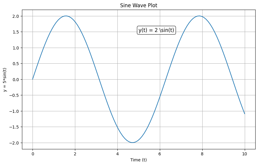
3D Plotting
# 3D plotting example
# Import 3D plotting toolkit for matplotlib (required for 3D surface plots)
from mpl_toolkits.mplot3d import Axes3D

fig = plt.figure(figsize=(10, 8)) # Create a new figure with a specific size
ax = fig.add_subplot(111, projection='3d')  # Add a 3D subplot to the figure

# Create meshgrid for 3D surface
x = np.linspace(-5, 5, 50)
y = np.linspace(-5, 5, 50)
X, Y = np.meshgrid(x, y)
Z = np.sin(np.sqrt(X**2 + Y**2))

# Create 3D surface plot
# Plot the 3D surface; cmap sets the color map, alpha sets transparency
# cmap='viridis' uses a blue-green-yellow color gradient for the surface
# alpha=0.8 makes the surface slightly transparent (1.0 is fully opaque)
surf = ax.plot_surface(X, Y, Z, cmap='viridis', alpha=0.8)
ax.set_xlabel('X')
ax.set_ylabel('Y')
ax.set_zlabel('Z')
ax.set_title('3D Surface Plot: Z = sin(√(X² + Y²))')
# Add color bar to indicate the mapping of colors to Z values
plt.colorbar(surf)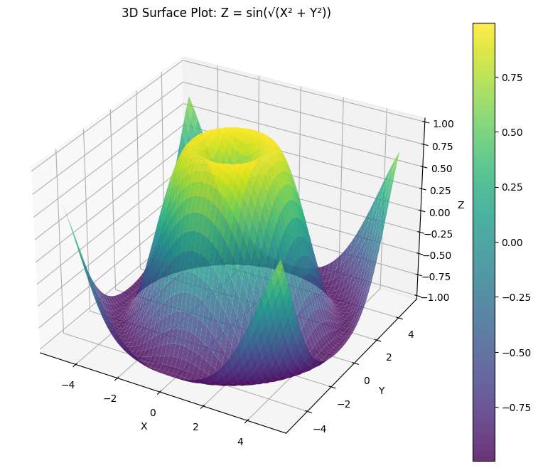
Plot with Custom Functions
In Python, you can define custom functions easily:
def ME564_fun(fxn_input):
    """Custom function that combines sine wave with random noise"""
    return 10 * np.sin(fxn_input * 10) + 5 * np.random.rand(*fxn_input.shape)

# Use the custom function
y_564 = ME564_fun(t)

plt.figure(figsize=(10, 6))
plt.plot(t, y_564, 'r-', linewidth=1.5)
plt.xlabel('Time (t), sec')
plt.ylabel('Function, f(t), -')
plt.title('Custom Function: 10*sin(10t) + 5*random')
plt.grid(True, alpha=0.3)
plt.show()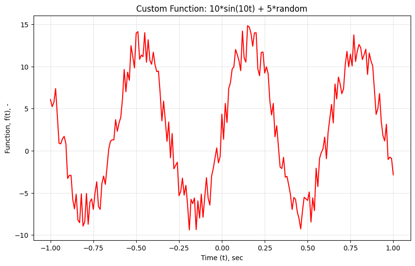
Task 4 – Debugging Techniques in Python
Effective debugging is crucial for engineering applications where accuracy is paramount. Python offers several powerful debugging tools and techniques that every engineer should know. We will go through two methods.
Method 1: Print statements and logging
# Method 1: Strategic Print Statements and Logging
# Example: Rotation Matrix Analysis in Robotics

def create_rotation_matrix(theta_deg, axis='z'):
    """
    Create a 3D rotation matrix with debugging prints

    Parameters:
    theta_deg: rotation angle in degrees
    axis: rotation axis ('x', 'y', or 'z')

    Returns:
    numpy.ndarray: 3x3 rotation matrix
    """
    print(f"DEBUG: Creating rotation matrix - angle={theta_deg}°, axis='{axis}'")

    # Convert angle to radians
    theta_rad = np.radians(theta_deg)
    print(f"DEBUG: Angle in radians: {theta_rad:.4f}")

    c = np.cos(theta_rad)
    s = np.sin(theta_rad)
    print(f"DEBUG: cos(θ)={c:.4f}, sin(θ)={s:.4f}")

    if axis == 'x':
        # 3D rotation about X-axis
        R = np.array([[1, 0, 0],
                      [0, c, -s],
                      [0, s, c]])
        print(f"DEBUG: Created 3D rotation matrix (X-axis)")
    elif axis == 'y':
        # 3D rotation about Y-axis
        R = np.array([[c, 0, s],
                      [0, 1, 0],
                      [-s, 0, c]])
        print(f"DEBUG: Created 3D rotation matrix (Y-axis)")
    elif axis == 'z':
        # 3D rotation about Z-axis
        R = np.array([[c, -s, 0],
                      [s, c, 0],
                      [0, 0, 1]])
        print(f"DEBUG: Created 3D rotation matrix (Z-axis)")
    else:
        raise ValueError("Axis must be 'x', 'y', or 'z'")

    print(f"DEBUG: Rotation matrix determinant: {np.linalg.det(R):.6f}")
    print(f"DEBUG: Matrix is orthogonal: {np.allclose(R @ R.T, np.eye(R.shape[0]))}")

    return R

# Test with a robot arm rotating 45 degrees about Z-axis
print("EXAMPLE: Rotating robot end-effector point about Z-axis\n")
R_z45 = create_rotation_matrix(45, axis='z')

# Original point in robot frame (100 mm, 50 mm, 0 mm)
point = np.array([100, 50, 0])
print(f"\nDEBUG: Original point: {point}")

# Rotate the point
rotated_point = R_z45 @ point
print(f"DEBUG: Rotated point: {rotated_point}")
print(f"DEBUG: Distance preserved: {np.linalg.norm(point):.2f} → {np.linalg.norm(rotated_point):.2f}")

print(f"\nFINAL RESULT: Point rotated 45° CCW about Z-axis")
print(f"  Before: ({point[0]:.1f}, {point[1]:.1f}, {point[2]:.1f}) mm")
print(f"  After:  ({rotated_point[0]:.1f}, {rotated_point[1]:.1f}, {rotated_point[2]:.1f}) mm")
EXAMPLE: Rotating robot end-effector point about Z-axis
DEBUG: Creating rotation matrix - angle=45°, axis='z'
DEBUG: Angle in radians: 0.7854
DEBUG: cos(θ)=0.7071, sin(θ)=0.7071
DEBUG: Created 3D rotation matrix (Z-axis)
DEBUG: Rotation matrix determinant: 1.000000
DEBUG: Matrix is orthogonal: True
DEBUG: Original point: [100 50 0]
DEBUG: Rotated point: [ 35.35533906 106.06601718 0. ]
DEBUG: Distance preserved: 111.80 → 111.80
FINAL RESULT: Point rotated 45° CCW about Z-axis
Before: (100.0, 50.0, 0.0) mm
After: (35.4, 106.1, 0.0) mm
Method 2: Python Debugger (pdb) - Interactive Debugging
The Python debugger allows you to pause execution, inspect variables, and step through code line by line.
Key pdb commands:
n(next): Execute next lines(step): Step into function callsl(list): Show current codep variable_name: Print variable valuepp variable_name: Pretty print variablec(continue): Continue executionq(quit): Quit debugger
# Method 2: Using pdb for interactive debugging
import numpy as np
import pdb

def rotate_point_2d(x, y, angle_deg):
    """
    Rotate a 2D point counterclockwise by angle_deg degrees around origin.
    Simple example to demonstrate pdb debugging.

    Parameters:
    x, y: point coordinates
    angle_deg: rotation angle in degrees

    Returns:
    tuple: (x_rotated, y_rotated)
    """

    # Uncomment the next line to pause execution and debug interactively


    # Step 1: Convert angle to radians
    angle_rad = np.radians(angle_deg)
    print(f"Step 1: angle_deg = {angle_deg}° → angle_rad = {angle_rad:.4f}")

    pdb.set_trace()  # Debugger will start here

    # Step 2: Calculate rotation components
    cos_a = np.cos(angle_rad)
    sin_a = np.sin(angle_rad)
    print(f"Step 2: cos(θ) = {cos_a:.4f}, sin(θ) = {sin_a:.4f}")

    # Step 3: Apply rotation matrix
    # [x']   [cos(θ)  -sin(θ)] [x]
    # [y'] = [sin(θ)   cos(θ)] [y]
    x_rotated = cos_a * x - sin_a * y
    y_rotated = sin_a * x + cos_a * y
    print(f"Step 3: ({x}, {y}) → ({x_rotated:.2f}, {y_rotated:.2f})")

    return x_rotated, y_rotated

# Example: Robot arm end-effector position
print("=== 2D Point Rotation (Robot End-Effector) ===\n")
print("Original point: (1.0, 0.0) - on X-axis")
print("Rotation: 90° counterclockwise\n")

x_new, y_new = rotate_point_2d(1.0, 0.0, 90)

print(f"\n=== RESULT ===")
print(f"After 90° rotation: ({x_new:.2f}, {y_new:.2f})")
print(f"Expected: (0.0, 1.0) - now on Y-axis")

# Try uncommenting pdb.set_trace() above to:
# - Type 'p x' to print x value
# - Type 'p angle_rad' to print angle_rad value
# - Type 'n' to execute next line
# - Type 'l' to list code around breakpoint
# - Type 'c' to continue execution
=== 2D Point Rotation (Robot End-Effector) ===
Original point: (1.0, 0.0) - on X-axis
Rotation: 90° counterclockwise
Step 1: angle_deg = 90° → angle_rad = 1.5708
> /tmp/ipython-input-2080816695.py(28)rotate_point_2d()
26
27 # Step 2: Calculate rotation components
---> 28 cos_a = np.cos(angle_rad)
29 sin_a = np.sin(angle_rad)
30 print(f"Step 2: cos(θ) = {cos_a:.4f}, sin(θ) = {sin_a:.4f}")
ipdb> p angle_rad
np.float64(1.5707963267948966)
--KeyboardInterrupt--
KeyboardInterrupt: Interrupted by user
Step 2: cos(θ) = 0.0000, sin(θ) = 1.0000
Step 3: (1.0, 0.0) → (0.00, 1.00)
=== RESULT ===
After 90° rotation: (0.00, 1.00)
Expected: (0.0, 1.0) - now on Y-axis
Task 5: Matrix Exponential and Logarithm for Rotation and Homogeneous Transformation Matrices
After understanding the basics for Python, we can now practice what we learned in lectures. In robot mechanics and control, we often need to convert between different representations of rotations and transformations. The matrix exponential and matrix logarithm provide powerful tools for this conversion.
1. Matrix Exponential and Logarithm for Rotation Matrices
For a 3×3 rotation matrix R, we can use the exponential map to generate rotations from a skew-symmetric matrix (rotation vector):
Exponential Map: from to , which can be obtained by
Input: Skew-symmetric matrix from unit rotation axis with rotation angle
Output: Three by three Rotation matrix R
In this task, we will implement Python functions to compute these maps for both rotation matrices and homogeneous transformation matrices, providing practical tools for robot mechanics calculations.
import numpy as np
# Helper function: Create skew-symmetric matrix from a 3D vector
def skew_symmetric(omega):
    """
    Create a 3x3 skew-symmetric matrix from a 3D vector.

    For a vector omega = [w1, w2, w3], creates:
    [omega] = [  0  -w3   w2]
              [ w3    0  -w1]
              [-w2   w1    0]

    Parameters:
    omega: 3D vector (numpy array or list)

    Returns:
    3x3 skew-symmetric matrix (numpy array)
    """
    omega = np.array(omega).flatten()
    if len(omega) != 3:
        raise ValueError("Input must be a 3D vector")

    return np.array([
        [0,         -omega[2],  omega[1]],
        [omega[2],   0,        -omega[0]],
        [-omega[1],  omega[0],  0]
    ])


def matrix_exp_so3(omega_hat_skew, theta):
    """
    Exponential map from so(3) to SO(3) using Rodrigues' formula.

    Computes: R = exp([omega_hat]*theta) = I + sin(theta)*[omega_hat] + (1-cos(theta))*[omega_hat]^2

    Parameters:
    omega_hat_skew: 3x3 skew-symmetric matrix of UNIT rotation axis (numpy array)
    theta: rotation angle in radians (scalar)

    Returns:
    R: 3x3 rotation matrix in SO(3)

    Example:
    >>> omega_hat = np.array([0, 0, 1])  # Unit vector along z-axis
    >>> omega_hat_skew = skew_symmetric(omega_hat)
    >>> R = matrix_exp_so3(omega_hat_skew, np.pi/2)  # 90 degree rotation about z
    """
    # Verify input is 3x3
    if omega_hat_skew.shape != (3, 3):
        raise ValueError("Input must be a 3x3 skew-symmetric matrix")

    # Check if matrix is skew-symmetric (within numerical tolerance)
    if not np.allclose(omega_hat_skew, -omega_hat_skew.T):
        raise ValueError("Input matrix must be skew-symmetric: [omega]^T = -[omega]")

    # Identity matrix
    I = np.eye(3)

    # Apply Rodrigues' formula
    # R = I + sin(theta)*[omega_hat] + (1-cos(theta))*[omega_hat]^2
    R = I + np.sin(theta) * omega_hat_skew + (1 - np.cos(theta)) * (omega_hat_skew @ omega_hat_skew)

    return R


def matrix_exp_so3_from_vector(omega_theta):
    """
    Exponential map from so(3) to SO(3) using exponential coordinates.

    This is a convenient wrapper that takes the rotation vector directly
    (where the magnitude is the angle and direction is the axis).

    Parameters:
    omega_theta: 3D rotation vector where ||omega_theta|| = theta (rotation angle)
                 and omega_theta/||omega_theta|| = omega_hat (unit rotation axis)

    Returns:
    R: 3x3 rotation matrix in SO(3)

    Example:
    >>> omega_theta = np.array([0, 0, np.pi/2])  # 90 deg rotation about z-axis
    >>> R = matrix_exp_so3_from_vector(omega_theta)
    """
    omega_theta = np.array(omega_theta).flatten()

    # Calculate rotation angle (magnitude of vector)
    theta = np.linalg.norm(omega_theta)

    # Handle special case: zero rotation
    if theta < 1e-10:
        return np.eye(3)

    # Extract unit rotation axis
    omega_hat = omega_theta / theta

    # Create skew-symmetric matrix
    omega_hat_skew = skew_symmetric(omega_hat)

    # Apply Rodrigues' formula
    return matrix_exp_so3(omega_hat_skew, theta)


# Test Example 1: Rotation about Z-axis by 90 degrees
print("=" * 60)
print("Example 1: Rotation about Z-axis by 90 degrees")
print("=" * 60)

# Define unit rotation axis (z-axis)
omega_hat = np.array([0, 0, 1])
theta = np.pi / 2  # 90 degrees in radians

# Create skew-symmetric matrix
omega_hat_skew = skew_symmetric(omega_hat)
print(f"\nUnit rotation axis (omega_hat): {omega_hat}")
print(f"Rotation angle (theta): {theta:.4f} rad = {np.degrees(theta):.1f}°")
print(f"\nSkew-symmetric matrix [omega_hat]:")
print(omega_hat_skew)

# Compute rotation matrix using exponential map
R_z90 = matrix_exp_so3(omega_hat_skew, theta)
print(f"\nRotation matrix R (from exponential map):")
print(R_z90)

# Verify it's a valid rotation matrix
print(f"\nVerification:")
print(f"  det(R) = {np.linalg.det(R_z90):.6f} (should be 1)")
print(f"  R*R^T = I? {np.allclose(R_z90 @ R_z90.T, np.eye(3))}")

# Test rotation on a point
point = np.array([1, 0, 0])  # Point on x-axis
rotated_point = R_z90 @ point
print(f"\nRotating point {point} by 90° about z-axis:")
print(f"  Result: [{rotated_point[0]:.4f}, {rotated_point[1]:.4f}, {rotated_point[2]:.4f}]")
print(f"  Expected: [0, 1, 0] (on y-axis)")


# Test Example 2: Using the vector wrapper function
print("\n" + "=" * 60)
print("Example 2: Using exponential coordinates (vector form)")
print("=" * 60)

# Rotation vector: direction = axis, magnitude = angle
omega_theta = np.array([0, np.pi/4, 0])  # 45° rotation about y-axis
print(f"\nRotation vector (omega*theta): {omega_theta}")
print(f"  Magnitude (angle): {np.linalg.norm(omega_theta):.4f} rad = {np.degrees(np.linalg.norm(omega_theta)):.1f}°")
print(f"  Direction (axis): {omega_theta / np.linalg.norm(omega_theta)}")

R_y45 = matrix_exp_so3_from_vector(omega_theta)
print(f"\nRotation matrix R:")
print(R_y45)

# Verify
print(f"\nVerification:")
print(f"  det(R) = {np.linalg.det(R_y45):.6f}")
print(f"  Orthogonal? {np.allclose(R_y45 @ R_y45.T, np.eye(3))}")
============================================================
Example 1: Rotation about Z-axis by 90 degrees
============================================================

Unit rotation axis (omega_hat): [0 0 1]
Rotation angle (theta): 1.5708 rad = 90.0°

Skew-symmetric matrix [omega_hat]:
[[ 0 -1  0]
 [ 1  0  0]
 [ 0  0  0]]

Rotation matrix R (from exponential map):
[[ 1.11022302e-16 -1.00000000e+00  0.00000000e+00]
 [ 1.00000000e+00  1.11022302e-16  0.00000000e+00]
 [ 0.00000000e+00  0.00000000e+00  1.00000000e+00]]

Verification:
  det(R) = 1.000000 (should be 1)
  R*R^T = I? True

Rotating point [1 0 0] by 90° about z-axis:
  Result: [0.0000, 1.0000, 0.0000]
  Expected: [0, 1, 0] (on y-axis)

============================================================
Example 2: Using exponential coordinates (vector form)
============================================================

Rotation vector (omega*theta): [0.         0.78539816 0.        ]
  Magnitude (angle): 0.7854 rad = 45.0°
  Direction (axis): [0. 1. 0.]

Rotation matrix R:
[[ 0.70710678  0.          0.70710678]
 [ 0.          1.          0.        ]
 [-0.70710678  0.          0.70710678]]

Verification:
  det(R) = 1.000000
  Orthogonal? True
Logarithm Map: from to , which can be obtained using the Algorithm on Page 87 of Mordern Robotics Textbook.
Input: Rotation matrix R
Output: Skew-symmetric matrix from unit rotation axis with rotation angle
def matrix_log_so3(R):
    """
    Logarithm map from SO(3) to so(3) using the algorithm from Modern Robotics textbook.

    Given R ∈ SO(3), find θ ∈ [0, π] and unit rotation axis ω ∈ ℝ³, ||ω|| = 1,
    such that R = exp([ω]θ).

    Algorithm:
    (a) If R = I, then θ = 0 and ω is undefined.
    (b) If tr(R) = -1, then θ = π. Use formula (3.60): ω = (1/√(2(1+r₁₁))) [1+r₁₁, r₂₁, r₃₁]ᵀ
    (c) Otherwise, θ = arccos((tr(R)-1)/2) and [ω] = (1/(2sinθ))(R - Rᵀ)

    Parameters:
    R: 3x3 rotation matrix (numpy array)

    Returns:
    omega_hat_skew: 3x3 skew-symmetric matrix [ω] = [ω]θ where ω is unit rotation axis
    theta: scalar rotation angle in radians
    omega_hat: 3D unit rotation axis vector (None if R=I)

    Example:
    >>> R = matrix_exp_so3_from_vector(np.array([0, 0, np.pi/2]))
    >>> omega_hat_skew, theta, omega_hat = matrix_log_so3(R)
    >>> print(f"Angle: {theta}, Axis: {omega_hat}")
    """

    # Verify input is 3x3
    if R.shape != (3, 3):
        raise ValueError("Input must be a 3x3 rotation matrix")

    # Verify it's a valid rotation matrix
    if not np.allclose(np.linalg.det(R), 1.0, atol=1e-6): #allclose checks if the determinant is close to 1 within a small tolerance
        raise ValueError(f"Input matrix determinant is {np.linalg.det(R):.6f}, not 1. Not a valid rotation matrix.")

    if not np.allclose(R @ R.T, np.eye(3), atol=1e-6):
        raise ValueError("Input matrix is not orthogonal (R @ R.T ≠ I). Not a valid rotation matrix.")

    # Case (a): If R = I, then θ = 0
    if np.allclose(R, np.eye(3), atol=1e-6):
        print("Case (a): R = I, so θ = 0 and ω is undefined")
        omega_hat_skew = np.zeros((3, 3))
        theta = 0.0
        omega_hat = None
        return omega_hat_skew, theta, omega_hat

    # Calculate trace of R, i.e., trace(r11 + r22 + r33)
    trace_R = np.trace(R)

    # Case (b): If tr(R) = -1, then θ = π
    if np.isclose(trace_R, -1.0, atol=1e-6):
        print("Case (b): tr(R) = -1, so θ = π")
        theta = np.pi

        # Use formula (3.60): ω = (1/√(2(1+r₁₁))) [1+r₁₁, r₂₁, r₃₁]ᵀ
        # where r₁₁ is R[0,0], r₂₁ is R[1,0], r₃₁ is R[2,0]
        r11 = R[0, 0]
        r21 = R[1, 0]
        r31 = R[2, 0]

        denominator = np.sqrt(2 * (1 + r11))

        if abs(denominator) < 1e-10:
            # Try formula (3.59) if (3.60) has numerical issues
            r12 = R[0, 1]
            r22 = R[1, 1]
            r32 = R[2, 1]
            denominator = np.sqrt(2 * (1 + r22))
            omega_hat = np.array([r12, 1 + r22, r32]) / denominator
        else:
            omega_hat = np.array([1 + r11, r21, r31]) / denominator

        omega_hat_skew = skew_symmetric(omega_hat)

        print(f"  Using formula (3.60): ω = {omega_hat}")
        return omega_hat_skew, theta, omega_hat

    # Case (c): Otherwise, use general formula
    print("Case (c): General case")

    # θ = arccos((tr(R) - 1) / 2)
    theta = np.arccos((trace_R - 1) / 2)

    # [ω] = (1/(2sinθ)) * (R - Rᵀ)
    sin_theta = np.sin(theta)

    if abs(sin_theta) < 1e-6:
        raise ValueError("sin(θ) is too close to zero. Numerical issue in logarithm computation.")

    omega_hat_skew = (1 / (2 * sin_theta)) * (R - R.T)

    # Extract ω from skew-symmetric matrix
    # For skew-symmetric matrix [ω] = [  0  -w3   w2]
    #                                 [ w3    0  -w1]
    #                                 [-w2   w1    0]
    # ω = [w1, w2, w3]
    omega_hat = np.array([omega_hat_skew[2, 1], omega_hat_skew[0, 2], omega_hat_skew[1, 0]])

    print(f"  θ = arccos((tr(R)-1)/2) = {theta:.6f} rad = {np.degrees(theta):.2f}°")
    print(f"  ω = {omega_hat}")

    return omega_hat_skew, theta, omega_hat


# Test Example 1: Logarithm of identity matrix
print("=" * 70)
print("Test 1: Logarithm of Identity Matrix (Case a)")
print("=" * 70)

R_identity = np.eye(3)
omega_skew_id, theta_id, omega_id = matrix_log_so3(R_identity)
print(f"Input: R = I₃ (identity matrix)")
print(f"Result: θ = {theta_id}, ω = {omega_id}")


# Test Example 2: Verify exponential-logarithm round trip (General case)
print("\n" + "=" * 70) # Print a separator line for clarity
print("Test 2: Round-trip Verification (exp → log → exp)")
print("=" * 70)

# Start with a rotation vector
omega_theta_original = np.array([0, 0, np.pi/3])  # 60° about z-axis
print(f"Original rotation vector: {omega_theta_original}")
print(f"  Angle: {np.linalg.norm(omega_theta_original):.6f} rad = {np.degrees(np.linalg.norm(omega_theta_original)):.2f}°")

# Compute exponential: rotation vector → rotation matrix
R_test = matrix_exp_so3_from_vector(omega_theta_original)
print(f"\nComputed rotation matrix R via exponential map:")
print(R_test)

# Compute logarithm: rotation matrix → rotation vector
omega_skew_test, theta_test, omega_hat_test = matrix_log_so3(R_test)
print(f"\nLogarithm of R:")
print(f"  Skew-symmetric matrix [ω]:")
print(omega_skew_test)
print(f"  Rotation angle: {theta_test:.6f} rad = {np.degrees(theta_test):.2f}°")
print(f"  Rotation axis: {omega_hat_test}")

# Reconstruct original rotation vector
omega_theta_recovered = omega_hat_test * theta_test
print(f"\nRecovered rotation vector: {omega_theta_recovered}")
print(f"Original rotation vector:  {omega_theta_original}")
print(f"Match? {np.allclose(omega_theta_recovered, omega_theta_original)}")

# Verify by applying exponential again
R_recovered = matrix_exp_so3_from_vector(omega_theta_recovered)
print(f"\nRe-applying exponential map:")
print(f"Original R matches recovered R? {np.allclose(R_test, R_recovered)}")


# Test Example 3: 180-degree rotation (Case b - tr(R) = -1)
print("\n" + "=" * 70)
print("Test 3: 180-Degree Rotation about [1, 0, 0] (Case b)")
print("=" * 70)

# 180° rotation about x-axis
omega_theta_180 = np.array([np.pi, 0, 0])
R_180 = matrix_exp_so3_from_vector(omega_theta_180)
print(f"Input rotation vector: {omega_theta_180}")
print(f"Rotation matrix:")
print(R_180)
print(f"Trace of R: {np.trace(R_180):.6f}")

omega_skew_180, theta_180, omega_hat_180 = matrix_log_so3(R_180)
print(f"\nLogarithm result:")
print(f"  θ = {theta_180:.6f} rad = {np.degrees(theta_180):.2f}°")
print(f"  ω = {omega_hat_180}")
print(f"  Recovered rotation vector: {omega_hat_180 * theta_180}")


# Test Example 4: Arbitrary rotation
print("\n" + "=" * 70)
print("Test 4: Arbitrary Rotation (45° about [1,1,1])")
print("=" * 70)

axis_arbitrary = np.array([1, 1, 1])
omega_hat_arb = axis_arbitrary / np.linalg.norm(axis_arbitrary)
theta_arbitrary = np.pi / 4  # 45°
omega_theta_arb = omega_hat_arb * theta_arbitrary

print(f"Original axis (normalized): {omega_hat_arb}")
print(f"Original angle: {theta_arbitrary:.6f} rad = {np.degrees(theta_arbitrary):.2f}°")

R_arb = matrix_exp_so3_from_vector(omega_theta_arb)
omega_skew_arb, theta_arb_recovered, omega_hat_arb_recovered = matrix_log_so3(R_arb)

print(f"\nRecovered axis: {omega_hat_arb_recovered}")
print(f"Recovered angle: {theta_arb_recovered:.6f} rad = {np.degrees(theta_arb_recovered):.2f}°")
print(f"Axis match? {np.allclose(omega_hat_arb, omega_hat_arb_recovered)}")
print(f"Angle match? {np.allclose(theta_arbitrary, theta_arb_recovered)}")
======================================================================
Test 1: Logarithm of Identity Matrix (Case a)
======================================================================
Case (a): R = I, so θ = 0 and ω is undefined
Input: R = I₃ (identity matrix)
Result: θ = 0.0, ω = None
======================================================================
Test 2: Round-trip Verification (exp → log → exp)
======================================================================
Original rotation vector: [0. 0. 1.04719755]
Angle: 1.047198 rad = 60.00°
Computed rotation matrix R via exponential map:
[[ 0.5 -0.8660254 0. ]
[ 0.8660254 0.5 0. ]
[ 0. 0. 1. ]]
Case (c): General case
θ = arccos((tr(R)-1)/2) = 1.047198 rad = 60.00°
ω = [0. 0. 1.]
Logarithm of R:
Skew-symmetric matrix [ω]:
[[ 0. -1. 0.]
[ 1. 0. 0.]
[ 0. 0. 0.]]
Rotation angle: 1.047198 rad = 60.00°
Rotation axis: [0. 0. 1.]
Recovered rotation vector: [0. 0. 1.04719755]
Original rotation vector: [0. 0. 1.04719755]
Match? True
Re-applying exponential map:
Original R matches recovered R? True
======================================================================
Test 3: 180-Degree Rotation about [1, 0, 0] (Case b)
======================================================================
Input rotation vector: [3.14159265 0. 0. ]
Rotation matrix:
[[ 1.0000000e+00 0.0000000e+00 0.0000000e+00]
[ 0.0000000e+00 -1.0000000e+00 -1.2246468e-16]
[ 0.0000000e+00 1.2246468e-16 -1.0000000e+00]]
Trace of R: -1.000000
Case (b): tr(R) = -1, so θ = π
Using formula (3.60): ω = [1. 0. 0.]
Logarithm result:
θ = 3.141593 rad = 180.00°
ω = [1. 0. 0.]
Recovered rotation vector: [3.14159265 0. 0. ]
======================================================================
Test 4: Arbitrary Rotation (45° about [1,1,1])
======================================================================
Original axis (normalized): [0.57735027 0.57735027 0.57735027]
Original angle: 0.785398 rad = 45.00°
Case (c): General case
θ = arccos((tr(R)-1)/2) = 0.785398 rad = 45.00°
ω = [0.57735027 0.57735027 0.57735027]
Recovered axis: [0.57735027 0.57735027 0.57735027]
Recovered angle: 0.785398 rad = 45.00°
Axis match? True
Angle match? True
2. Matrix Exponential and Logarithm for Homogeneous Transformation Matrices
We can perform the similar transformation for Homogeneous Transformation Matrices. Specifically, for SE(3) (Special Euclidean Group in 3D), a homogeneous transformation matrix combines rotation and translation:
Exponential Map: where is a 4×4 matrix from the screw :
Input:
Output: Homogeneous transformation T
def matrix_exp_se3(S, theta):
    """
    Exponential map from se(3) to SE(3) using screw axis formulation.

    Given screw axis S = [S_omega, S_v] and angle theta, compute:
    T = exp([S] theta) = [[R, p], [0, 1]]

    If ||S_omega|| = 0 (pure translation):
        R = I, p = S_v * theta
    Otherwise:
        R = exp([omega_hat] theta)
        p = (I*theta + (1-cos(theta))[omega_hat] + (theta - sin(theta))[omega_hat]^2) S_v

    Parameters:
    S: 6D screw axis array [S_omega (3,), S_v (3,)]
    theta: scalar joint displacement

    Returns:
    T: 4x4 homogeneous transformation matrix in SE(3)
    """
    S = np.array(S).flatten()
    if S.shape[0] != 6:
        raise ValueError("S must be a 6D vector: [S_omega, S_v]")

    S_omega = S[:3]
    S_v = S[3:]

    omega_norm = np.linalg.norm(S_omega)
    I = np.eye(3)

    if omega_norm < 1e-10:
        # Pure translation
        R = I
        p = S_v * theta
    else:
        # Rotation + translation
        omega_hat = S_omega / omega_norm
        omega_hat_skew = skew_symmetric(omega_hat)

        R = matrix_exp_so3(omega_hat_skew, theta)

        V = (
            I * theta
            + (1 - np.cos(theta)) * omega_hat_skew
            + (theta - np.sin(theta)) * (omega_hat_skew @ omega_hat_skew)
        )
        p = V @ S_v

    T = np.eye(4)
    T[:3, :3] = R
    T[:3, 3] = p

    return T


# Test Example 1: Pure translation
print("=" * 70)
print("SE(3) Exponential Map - Test 1: Pure Translation")
print("=" * 70)

S_translation = np.array([0, 0, 0, 1, 2, 3])
theta_translation = 0.5
T_translation = matrix_exp_se3(S_translation, theta_translation)

print(f"S = {S_translation}, theta = {theta_translation}")
print("T =")
print(T_translation)


# Test Example 2: Rotation about z-axis with translation
print("\n" + "=" * 70)
print("SE(3) Exponential Map - Test 2: Rotation + Translation")
print("=" * 70)

S_screw = np.array([0, 0, 1, 1, 0, 0])  # omega = z-axis, v = x-axis

theta_screw = np.pi / 4  # 45 degrees
T_screw = matrix_exp_se3(S_screw, theta_screw)

print(f"S = {S_screw}, theta = {theta_screw:.4f} rad")
print("T =")
print(T_screw)

# Verify rotation part is orthogonal
print(f"\nRotation det(R) = {np.linalg.det(T_screw[:3, :3]):.6f}")
print(f"Rotation orthogonal? {np.allclose(T_screw[:3, :3] @ T_screw[:3, :3].T, np.eye(3))}")
======================================================================
SE(3) Exponential Map - Test 1: Pure Translation
======================================================================
S = [0 0 0 1 2 3], theta = 0.5
T =
[[1.  0.  0.  0.5]
 [0.  1.  0.  1. ]
 [0.  0.  1.  1.5]
 [0.  0.  0.  1. ]]

======================================================================
SE(3) Exponential Map - Test 2: Rotation + Translation
======================================================================
S = [0 0 1 1 0 0], theta = 0.7854 rad
T =
[[ 0.70710678 -0.70710678  0.          0.70710678]
 [ 0.70710678  0.70710678  0.          0.29289322]
 [ 0.          0.          1.          0.        ]
 [ 0.          0.          0.          1.        ]]

Rotation det(R) = 1.000000
Rotation orthogonal? True
Logarithm Map:
Input: Homogeneous transformation T
Output: expoential coordinates
The following code is based on the algorithm on page 106 in Modern Robotics textbook.
def matrix_log_se3(T):
    """
    Logarithm map from SE(3) to se(3) using the Modern Robotics algorithm.

    Given T = [[R, p], [0, 1]], find theta in [0, pi] and screw axis S = (S_omega, S_v)
    such that exp([S] theta) = T.

    Algorithm:
    (a) If R = I: set S_omega = 0, S_v = p / ||p||, and theta = ||p||.
    (b) Otherwise: use log on SO(3) to get S_omega (unit) and theta, then
        S_v = G_inv(theta) * p
        G_inv(theta) = (1/theta) I - (1/2) [S_omega] + (1/theta - 1/2 cot(theta/2)) [S_omega]^2

    Parameters:
    T: 4x4 homogeneous transformation matrix (numpy array)

    Returns:
    S_omega: 3D unit rotation axis (or zero vector for pure translation)
    S_v: 3D linear velocity component of screw axis
    theta: scalar magnitude
    S_theta: 6D exponential coordinates = [S_omega, S_v] * theta
    """
    T = np.array(T)
    if T.shape != (4, 4):
        raise ValueError("Input T must be a 4x4 homogeneous transformation matrix")

    R = T[:3, :3]
    p = T[:3, 3]

    # Case (a): Pure translation (R = I)
    if np.allclose(R, np.eye(3), atol=1e-6):
        theta = np.linalg.norm(p)
        if theta < 1e-10:
            # Identity transform
            S_omega = np.zeros(3)
            S_v = np.zeros(3)
            S_theta = np.zeros(6)
            return S_omega, S_v, theta, S_theta

        S_omega = np.zeros(3)
        S_v = p / theta
        S_theta = np.hstack([S_omega, S_v]) * theta
        return S_omega, S_v, theta, S_theta

    # Case (b): General case with rotation
    omega_hat_skew, theta, omega_hat = matrix_log_so3(R)
    S_omega = omega_hat

    # Compute G_inv(theta)
    I = np.eye(3)
    half_theta = 0.5 * theta
    cot_half_theta = np.cos(half_theta) / np.sin(half_theta)

    G_inv = (
        (1.0 / theta) * I
        - 0.5 * omega_hat_skew
        + (1.0 / theta - 0.5 * cot_half_theta) * (omega_hat_skew @ omega_hat_skew)
    )

    S_v = G_inv @ p
    S_theta = np.hstack([S_omega, S_v]) * theta

    return S_omega, S_v, theta, S_theta


# Test Example 1: Pure translation
print("=" * 70)
print("SE(3) Logarithm Map - Test 1: Pure Translation")
print("=" * 70)

T_translation = np.eye(4)
T_translation[:3, 3] = np.array([1.0, 2.0, 3.0])

S_omega, S_v, theta, S_theta = matrix_log_se3(T_translation)
print("T =")
print(T_translation)
print(f"S_omega = {S_omega}")
print(f"S_v = {S_v}")
print(f"theta = {theta:.6f}")
print(f"S_theta = {S_theta}")


# Test Example 2: Rotation + translation (round-trip check)
print("\n" + "=" * 70)
print("SE(3) Logarithm Map - Test 2: Rotation + Translation")
print("=" * 70)

S_test = np.array([0, 0, 1, 1, 0, 0])
theta_test = np.pi / 4
T_test = matrix_exp_se3(S_test, theta_test)

S_omega2, S_v2, theta2, S_theta2 = matrix_log_se3(T_test)
print("T =")
print(T_test)
print(f"S_omega = {S_omega2}")
print(f"S_v = {S_v2}")
print(f"theta = {theta2:.6f}")
print(f"S_theta = {S_theta2}")

# Reconstruct T from recovered screw axis
T_recovered = matrix_exp_se3(np.hstack([S_omega2, S_v2]), theta2)
print(f"\nRecovered T matches original? {np.allclose(T_test, T_recovered)}")
======================================================================
SE(3) Logarithm Map - Test 1: Pure Translation
======================================================================
T =
[[1. 0. 0. 1.]
 [0. 1. 0. 2.]
 [0. 0. 1. 3.]
 [0. 0. 0. 1.]]
S_omega = [0. 0. 0.]
S_v = [0.26726124 0.53452248 0.80178373]
theta = 3.741657
S_theta = [0. 0. 0. 1. 2. 3.]

======================================================================
SE(3) Logarithm Map - Test 2: Rotation + Translation
======================================================================
Case (c): General case
  θ = arccos((tr(R)-1)/2) = 0.785398 rad = 45.00°
  ω = [0. 0. 1.]
T =
[[ 0.70710678 -0.70710678  0.          0.70710678]
 [ 0.70710678  0.70710678  0.          0.29289322]
 [ 0.          0.          1.          0.        ]
 [ 0.          0.          0.          1.        ]]
S_omega = [0. 0. 1.]
S_v = [1.00000000e+00 2.29934717e-17 0.00000000e+00]
theta = 0.785398
S_theta = [0.00000000e+00 0.00000000e+00 7.85398163e-01 7.85398163e-01
 1.80590304e-17 0.00000000e+00]

Recovered T matches original? True
HW Problems
Now that you’ve learned the basics, practice the following problems. Work through them step by step, using the debugging techniques you’ve learned. You need to submit your solutions to these HW problems with your source code.
Problem 1: Basic Python Syntax and Control Flow
In this problem, you will analyze material properties for design selection.
Task: Write a program that:
Creates a dictionary of materials with their properties (density, yield strength, cost per kg)
Finds the material with the highest strength-to-weight ratio
Determines which materials are suitable for a given application (yield strength > 200 MPa, cost < $10/kg)
Uses proper error handling for invalid inputs
Given data:
Steel: density=7850 kg/m³, yield=250 MPa, cost=$2/kg
Aluminum: density=2700 kg/m³, yield=70 MPa, cost=$8/kg
Titanium: density=4500 kg/m³, yield=880 MPa, cost=$30/kg
Carbon Fiber: density=1600 kg/m³, yield=600 MPa, cost=$50/kg
# Problem 1 Solution Space
# Write your solution here

# Hint: Start by creating the materials dictionary
materials = {
    # Fill in the material properties
}

# Your code here...
Problem 2: NumPy Arrays and Mathematical Operations
In this problem, you will analyze experimental strain gauge data and plot them.
Task: Given strain measurements from 5 gauges over 10 time steps:
Create a 2D NumPy array (10 time steps × 5 gauges) with realistic strain data
Calculate the maximum, minimum, and average strain for each gauge
Find the time step where the maximum overall strain occurred
Calculate the stress using σ = E × ε (E = 200 GPa for steel)
Plot strain vs time for all gauges on the same plot with different colors
Add proper labels, legend, and title
Hints:
Use
np.random.normal()to generate realistic strain data around 0.001 (1000 microstrain)Use
np.argmax()to find indices of maximum valuesRemember to convert units properly (strain is dimensionless, stress in Pa)
# Problem 2 Solution Space
import numpy as np
import matplotlib.pyplot as plt

# Create time array
time = np.linspace(0, 10, 10)  # 10 time steps from 0 to 10 seconds

# Generate strain data (your code here)
# Hint: strain_data = np.random.normal(loc=0.001, scale=0.0002, size=(10, 5))

# Your analysis code here...
Problem 3: Matrix Exponential Practice (Task 5)
Use the functions from Task 5 to compute matrix exponentials. Keep the calculations simple and verify results.
Rotation Matrix (SO(3))
Given: Unit rotation axis with angle .
Step 1: Compute the rotation matrix using
matrix_exp_so3_from_vector(exponential map).Step 2: Verify that is a valid rotation matrix (check and ).
Step 3: Apply the logarithm map using
matrix_log_so3to recover and .Step 4: Verify that the recovered rotation axis and angle match the original values.
Homogeneous Transformation (SE(3))
Given: Screw axis with .
Step 1: Compute the transformation matrix using
matrix_exp_se3(exponential map).Step 2: Verify that the rotation part is orthogonal and print the translation vector.
Step 3: Apply the logarithm map using
matrix_log_se3to recover and .Step 4: Verify that the recovered screw axis and angle match the original values (compute from the recovered values).