
In this lab, you will design and implement feedback controllers for robotic manipulators of increasing complexity — from a single-joint arm to a 6-DOF industrial robot. The lab builds progressively: controllers derived analytically in Tasks 1–2 are extended to multi-link robots in Tasks 3–4 using MuJoCo as the physics simulator. The final Problems section asks you to apply these ideas independently to a new 3R spatial robot.
Learning Objectives
By the end of this lab, you should be able to:
Derive and simulate single-joint controllers — implement speed (PI) and position (PD) feedback control for a 1R arm using an analytical dynamics model, and analyze closed-loop stability.
Apply computed torque control (CTC) — implement the feedforward + feedback computed torque law that cancels nonlinear dynamics and produces decoupled linear error dynamics for exact trajectory tracking.
Use MuJoCo for robot simulation — interface with MuJoCo’s dynamics API to compute mass matrices, bias forces, and Jacobians without deriving them analytically.
Extend CTC to multi-link robots — generalize computed torque control from a 1R arm to a 2R planar robot and a 6-DOF UR5, in both joint space and operational (Cartesian) space.
Compare joint-space and operational-space control — understand the relationship between joint-space CTC, operational-space CTC, and IK + joint-space CTC.
Design controllers for a new robot — implement PD and computed torque controllers for a 3R spatial robot, tune gains, and evaluate performance on reaching and trajectory tracking tasks.
!pip install mujoco mediapy numpy scipy
import os
import mujoco
import mediapy as media
import numpy as np
from IPython.display import clear_output
clear_output()
Task 1: Control of a Single Joint Robotic Arm Using Analytical Models
Dynamics Model
Consider a single motor attached to a single rigid link. Let be the motor torque and the joint angle. Rotational friction is modeled as a viscous damping force (Eq. 11.20):
Adding the friction torque to the basic equation of motion gives the full model (Eq. 11.21):
which can be written compactly as (Eq. 11.22):
where contains all state-dependent terms. Rearranging for simulation:
Variable definitions:
: scalar rotational inertia [kg·m²]
: link mass [kg]
: distance from joint axis to center of mass [m]
: viscous friction coefficient [N·m·s/rad]
: gravitational acceleration [m/s²]
Two models used throughout this task (textbook parameters: kg·m², kg, m, N·m·s/rad):
| Model | Gravity | Equation of Motion |
|---|---|---|
| Horizontal | ||
| Vertical |
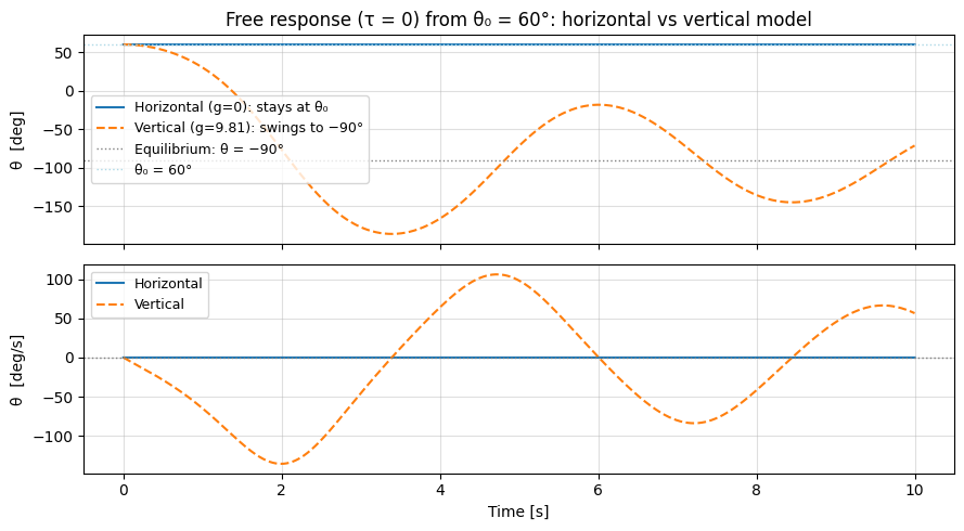
The horizontal model reduces to a first-order system in , useful for speed control. The vertical model adds a nonlinear gravity load that controllers must compensate.
import numpy as np
from scipy.integrate import solve_ivp
import matplotlib.pyplot as plt

# -------------------------------------------------------
# Single-Joint Dynamics Parameters (textbook values)
# -------------------------------------------------------
# Full model (Eq. 11.21):  τ = M*θ̈ + m*g*r*cos(θ) + b*θ̇
#   vertical   (with gravity):  τ = M*θ̈ + m*g*r*cos(θ) + b*θ̇
#   horizontal (g = 0):         τ = M*θ̈ + b*θ̇

M_link = 0.5   # rotational inertia [kg·m²]
m_link = 1.0   # link mass [kg]
r_link = 0.1   # distance from joint axis to CoM [m]
b_link = 0.1   # viscous friction coefficient [N·m·s/rad]
g_acc  = 9.81  # gravitational acceleration [m/s²]


class SingleJointModel:
    """
    Dynamics model for a single revolute joint with viscous friction.

    Full equation of motion (Eq. 11.21):
        τ = M*θ̈ + m*g*r*cos(θ) + b*θ̇

    Rearranged for simulation:
        θ̈ = (τ - m*g*r*cos(θ) - b*θ̇) / M

    Setting g=0 gives the horizontal (gravity-free) model:
        θ̈ = (τ - b*θ̇) / M

    Parameters
    ----------
    M : float – rotational inertia [kg·m²]
    m : float – link mass [kg]
    r : float – distance from joint axis to CoM [m]
    b : float – viscous friction coefficient [N·m·s/rad]
    g : float – gravitational acceleration (0 for horizontal)
    """

    def __init__(self, M, m, r, b, g=0.0):
        self.M = M
        self.m = m
        self.r = r
        self.b = b
        self.g = g

    def h(self, theta, theta_dot):
        """State-dependent torque h(θ, θ̇) = m*g*r*cos(θ) + b*θ̇  [N·m]"""
        return self.m * self.g * self.r * np.cos(theta) + self.b * theta_dot

    def _ode(self, t, state, tau_func):
        """
        ODE right-hand side.
        state = [θ, θ̇]  →  returns [θ̇, θ̈]
        """
        theta, theta_dot = state
        tau = tau_func(t, state)
        theta_ddot = (tau - self.h(theta, theta_dot)) / self.M
        return [theta_dot, theta_ddot]

    def simulate(self, tau_func, t_span, state0, dt=0.001):
        """
        Simulate the joint dynamics with RK45.

        Parameters
        ----------
        tau_func : callable(t, state) → float   applied torque [N·m]
        t_span   : (t0, tf)                     simulation time window [s]
        state0   : [θ0, θ̇0]                    initial conditions
        dt       : float                         output time step [s]

        Returns
        -------
        t      : (N,) array – time [s]
        theta  : (N,) array – joint angle [rad]
        dtheta : (N,) array – joint velocity [rad/s]
        """
        t_eval = np.arange(t_span[0], t_span[1], dt)
        sol = solve_ivp(
            self._ode,
            t_span,
            state0,
            args=(tau_func,),
            t_eval=t_eval,
            method="RK45",
            rtol=1e-6,
            atol=1e-8,
        )
        return sol.t, sol.y[0], sol.y[1]


# -------------------------------------------------------
# Instantiate both models
# -------------------------------------------------------
model_horizontal = SingleJointModel(M=M_link, m=m_link, r=r_link, b=b_link, g=0.0)
model_vertical   = SingleJointModel(M=M_link, m=m_link, r=r_link, b=b_link, g=g_acc)

max_gravity = model_vertical.m * model_vertical.g * model_vertical.r
print(f"Max gravity torque: m·g·r = {max_gravity:.3f} N·m  (at θ=0)")

# -------------------------------------------------------
# Sanity check: free response from θ₀ = 60° (τ = 0)
#
# Horizontal: no restoring force → friction damps θ̇ to zero, θ stays near θ₀
# Vertical:   gravity acts as restoring force → pendulum oscillation settling at θ = -π/2
# -------------------------------------------------------
tau_zero = lambda t, state: 0.0
theta0   = np.pi / 3          # initial angle: 60°
state0   = [theta0, 0.0]      # start from rest
t_span   = (0.0, 10.0)

t_h, th_h, dth_h = model_horizontal.simulate(tau_zero, t_span, state0)
t_v, th_v, dth_v = model_vertical.simulate(tau_zero, t_span, state0)

fig, axes = plt.subplots(2, 1, figsize=(9, 5), sharex=True)

axes[0].plot(t_h, np.degrees(th_h), label="Horizontal (g=0): stays at θ₀")
axes[0].plot(t_v, np.degrees(th_v), label="Vertical (g=9.81): swings to −90°", linestyle="--")
axes[0].axhline(-90, color="gray", linestyle=":", lw=1, label="Equilibrium: θ = −90°")
axes[0].axhline(np.degrees(theta0), color="lightblue", linestyle=":", lw=1, label=f"θ₀ = {np.degrees(theta0):.0f}°")
axes[0].set_ylabel("θ  [deg]")
axes[0].legend(fontsize=9)
axes[0].set_title("Free response (τ = 0) from θ₀ = 60°: horizontal vs vertical model")
axes[0].grid(True, alpha=0.4)

axes[1].plot(t_h, np.degrees(dth_h), label="Horizontal")
axes[1].plot(t_v, np.degrees(dth_v), label="Vertical", linestyle="--")
axes[1].axhline(0, color="gray", linestyle=":", lw=1)
axes[1].set_ylabel("θ̇  [deg/s]")
axes[1].set_xlabel("Time [s]")
axes[1].legend(fontsize=9)
axes[1].grid(True, alpha=0.4)

plt.tight_layout()
plt.show()
Max gravity torque: m·g·r = 0.981 N·m (at θ=0)
Speed Control: First-Order System
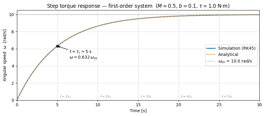
Using the horizontal model (), the equation of motion in terms of angular speed is:
This is a first-order linear ODE in . For a constant (step) torque input , the analytical solution is:
where:
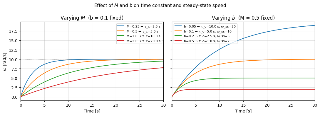
: steady-state speed (set by friction, independent of inertia)
: time constant: time for to reach of
A larger inertia slows the response; a larger friction reduces both the time constant and the steady-state speed.
# -------------------------------------------------------
# Speed Control: First-Order System (horizontal model)
# Input: constant torque τ   Output: angular speed ω = θ̇
# -------------------------------------------------------

tau_step = 1.0   # step torque input [N·m]
t_span   = (0.0, 30.0)
state0   = [0.0, 0.0]   # [θ0, ω0] — start from rest

# Simulate with the horizontal model
tau_func = lambda t, state: tau_step
t_sim, _, omega_sim = model_horizontal.simulate(tau_func, t_span, state0)

# -------------------------------------------------------
# Analytical first-order step response
# ω(t) = ω_ss * (1 - exp(-t / τ_c))
# -------------------------------------------------------
tau_c   = model_horizontal.M / model_horizontal.b   # time constant [s]
omega_ss = tau_step / model_horizontal.b             # steady-state speed [rad/s]
omega_analytical = omega_ss * (1 - np.exp(-t_sim / tau_c))

print(f"Time constant  τ_c  = M / b = {model_horizontal.M} / {model_horizontal.b} = {tau_c:.2f} s")
print(f"Steady-state speed  ω_ss = τ / b = {tau_step} / {model_horizontal.b} = {omega_ss:.2f} rad/s")
print(f"At t = τ_c:  ω = {omega_ss * (1 - np.exp(-1)):.3f} rad/s  ({(1-np.exp(-1))*100:.1f}% of ω_ss)")

# -------------------------------------------------------
# Plot: illustrate time constant concept
# -------------------------------------------------------
fig, ax = plt.subplots(figsize=(9, 4))

ax.plot(t_sim, omega_sim,         color="tab:blue",   lw=2,   label="Simulation (RK45)")
ax.plot(t_sim, omega_analytical,  color="tab:orange", lw=1.5, linestyle="--", label="Analytical")
ax.axhline(omega_ss, color="gray", linestyle=":",  lw=1.5, label=f"$\\omega_{{ss}}$ = {omega_ss:.1f} rad/s")

# Mark the time constant point
omega_tc = omega_ss * (1 - np.exp(-1))
ax.annotate(
    f"$t = \\tau_c = {tau_c:.0f}$ s\n$\\omega = 0.632\\,\\omega_{{ss}}$",
    xy=(tau_c, omega_tc),
    xytext=(tau_c + 1.5, omega_tc - 1.5),
    arrowprops=dict(arrowstyle="->", color="black"),
    fontsize=10,
)
ax.plot(tau_c, omega_tc, "ko", markersize=6)

# Mark multiples of τ_c with vertical dashed lines
for k in range(1, 6):
    ax.axvline(k * tau_c, color="lightgray", linestyle="--", lw=0.8)
    ax.text(k * tau_c + 0.3, 0.3, f"$t={k}\\tau_c$", fontsize=8, color="gray")

ax.set_xlabel("Time [s]")
ax.set_ylabel("Angular speed  ω  [rad/s]")
ax.set_title(f"Step torque response — first-order system  "
             f"($M={model_horizontal.M}$, $b={model_horizontal.b}$, $\\tau={tau_step}$ N·m)")
ax.legend()
ax.grid(True, alpha=0.4)
ax.set_xlim(t_span)
ax.set_ylim(bottom=0)

plt.tight_layout()
plt.show()

# -------------------------------------------------------
# Effect of varying M and b on the time constant
# -------------------------------------------------------
fig, axes = plt.subplots(1, 2, figsize=(11, 4), sharey=True)

# Vary M, fix b
for M_val in [0.25, 0.5, 1.0, 2.0]:
    mod = SingleJointModel(M=M_val, m=m_link, r=r_link, b=b_link, g=0.0)
    tc  = M_val / b_link
    oss = tau_step / b_link
    omega = oss * (1 - np.exp(-t_sim / tc))
    axes[0].plot(t_sim, omega, label=f"M={M_val} → τ_c={tc:.1f} s")
axes[0].axhline(tau_step / b_link, color="gray", linestyle=":", lw=1)
axes[0].set_xlabel("Time [s]"); axes[0].set_ylabel("ω [rad/s]")
axes[0].set_title(f"Varying $M$  (b = {b_link} fixed)")
axes[0].legend(fontsize=8); axes[0].grid(True, alpha=0.4)
axes[0].set_xlim(0, 30)

# Vary b, fix M
for b_val in [0.05, 0.1, 0.2, 0.5]:
    mod = SingleJointModel(M=M_link, m=m_link, r=r_link, b=b_val, g=0.0)
    tc  = M_link / b_val
    oss = tau_step / b_val
    omega = oss * (1 - np.exp(-t_sim / tc))
    axes[1].plot(t_sim, omega, label=f"b={b_val} → τ_c={tc:.1f} s, ω_ss={oss:.0f}")
axes[1].set_xlabel("Time [s]")
axes[1].set_title(f"Varying $b$  (M = {M_link} fixed)")
axes[1].legend(fontsize=8); axes[1].grid(True, alpha=0.4)
axes[1].set_xlim(0, 30)

plt.suptitle("Effect of $M$ and $b$ on time constant and steady-state speed", fontsize=11)
plt.tight_layout()
plt.show()
Time constant τ_c = M / b = 0.5 / 0.1 = 5.00 s
Steady-state speed ω_ss = τ / b = 1.0 / 0.1 = 10.00 rad/s
At t = τ_c: ω = 6.321 rad/s (63.2% of ω_ss)
Position PD Control: Second-Order System
The PD control law commands torque based on position and velocity error:
Substituting into the horizontal model () and defining error with constant setpoint () gives the closed-loop error dynamics (Eq. 11.25):
Rewriting in standard second-order form (Eq. 11.26):
where the natural frequency and damping ratio are:
Inverting these to solve for gains:
Two design methods:
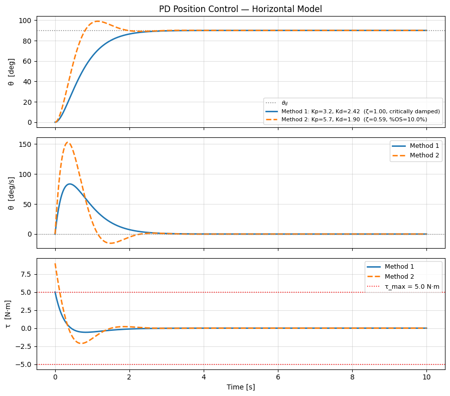
Method 1: Actuator-limited , critically damped : The peak torque occurs at : . Choose so the initial torque equals the actuator limit , then choose for (critically damped, no overshoot):
Method 2: Specification-driven design: Given a desired percent overshoot and settling time , solve for and :
then compute and .
# -------------------------------------------------------
# Position PD Control — Horizontal Model (g = 0)
# -------------------------------------------------------

theta_d = np.pi / 2   # desired position: 90° [rad]
theta_0 = 0.0         # initial position [rad]
t_span  = (0.0, 10.0)
state0  = [theta_0, 0.0]

# -------------------------------------------------------
# Method 1: Kp set by actuator limit, Kd for ζ = 1
# -------------------------------------------------------
tau_max = 5.0   # actuator torque limit [N·m]
e0      = theta_d - theta_0   # initial error [rad]

Kp1 = tau_max / e0                      # largest Kp within actuator limit
Kd1 = 2 * np.sqrt(Kp1 * M_link) - b_link   # ζ = 1 → critically damped
zeta1  = (b_link + Kd1) / (2 * np.sqrt(Kp1 * M_link))
omega_n1 = np.sqrt(Kp1 / M_link)

print("=== Method 1: Actuator-limited Kp, critically damped ===")
print(f"  Kp = τ_max / e0 = {tau_max} / {e0:.3f} = {Kp1:.3f} N·m/rad")
print(f"  Kd = 2√(Kp·M) - b = {Kd1:.3f} N·m·s/rad")
print(f"  → ωn = {omega_n1:.3f} rad/s,  ζ = {zeta1:.3f}  (critically damped, no overshoot)")
print(f"  Peak torque at t=0: {Kp1 * e0:.2f} N·m  (= τ_max ✓)")

# -------------------------------------------------------
# Method 2: Specification-driven — %OS and settling time
# -------------------------------------------------------
percent_OS = 10.0   # desired percent overshoot [%]
t_settle   = 2.0    # desired settling time (2% criterion) [s]

ln_os  = np.log(percent_OS / 100.0)
zeta2  = -ln_os / np.sqrt(np.pi**2 + ln_os**2)
omega_n2 = 4.0 / (zeta2 * t_settle)    # 2% settling time approximation

Kp2 = M_link * omega_n2**2
Kd2 = 2 * zeta2 * omega_n2 * M_link - b_link

print("\n=== Method 2: Specification-driven (%OS, settling time) ===")
print(f"  Desired: %OS = {percent_OS}%,  t_settle = {t_settle} s")
print(f"  → ζ = {zeta2:.3f},  ωn = {omega_n2:.3f} rad/s")
print(f"  Kp = M·ωn² = {Kp2:.3f} N·m/rad")
print(f"  Kd = 2ζωn·M - b = {Kd2:.3f} N·m·s/rad")
print(f"  Peak torque at t=0: {Kp2 * e0:.2f} N·m")

# -------------------------------------------------------
# PD controller simulation
# -------------------------------------------------------
def make_pd_controller(Kp, Kd, theta_d):
    """Return a tau_func implementing τ = Kp*(θd-θ) + Kd*(0-θ̇)"""
    def tau_func(t, state):
        theta, theta_dot = state
        return Kp * (theta_d - theta) + Kd * (0.0 - theta_dot)
    return tau_func

t1, th1, dth1 = model_horizontal.simulate(make_pd_controller(Kp1, Kd1, theta_d), t_span, state0)
t2, th2, dth2 = model_horizontal.simulate(make_pd_controller(Kp2, Kd2, theta_d), t_span, state0)

# Compute torque history for each method
tau1 = np.array([Kp1*(theta_d - th) - Kd1*dth for th, dth in zip(th1, dth1)])
tau2 = np.array([Kp2*(theta_d - th) - Kd2*dth for th, dth in zip(th2, dth2)])

# -------------------------------------------------------
# Plot
# -------------------------------------------------------
fig, axes = plt.subplots(3, 1, figsize=(9, 8), sharex=True)

# Position
axes[0].axhline(np.degrees(theta_d), color="gray", linestyle=":", lw=1.2, label="$\\theta_d$")
axes[0].plot(t1, np.degrees(th1), lw=2,
             label=f"Method 1: Kp={Kp1:.1f}, Kd={Kd1:.2f}  (ζ={zeta1:.2f}, critically damped)")
axes[0].plot(t2, np.degrees(th2), lw=2, linestyle="--",
             label=f"Method 2: Kp={Kp2:.1f}, Kd={Kd2:.2f}  (ζ={zeta2:.2f}, %OS={percent_OS}%)")
axes[0].set_ylabel("θ  [deg]")
axes[0].legend(fontsize=8)
axes[0].set_title("PD Position Control — Horizontal Model")
axes[0].grid(True, alpha=0.4)

# Velocity
axes[1].plot(t1, np.degrees(dth1), lw=2,             label="Method 1")
axes[1].plot(t2, np.degrees(dth2), lw=2, linestyle="--", label="Method 2")
axes[1].axhline(0, color="gray", linestyle=":", lw=1)
axes[1].set_ylabel("θ̇  [deg/s]")
axes[1].legend(fontsize=9)
axes[1].grid(True, alpha=0.4)

# Torque
axes[2].plot(t1, tau1, lw=2,             label="Method 1")
axes[2].plot(t2, tau2, lw=2, linestyle="--", label="Method 2")
axes[2].axhline( tau_max, color="red", linestyle=":", lw=1.2, label=f"τ_max = {tau_max} N·m")
axes[2].axhline(-tau_max, color="red", linestyle=":", lw=1.2)
axes[2].set_ylabel("τ  [N·m]")
axes[2].set_xlabel("Time [s]")
axes[2].legend(fontsize=9)
axes[2].grid(True, alpha=0.4)

plt.tight_layout()
plt.show()
=== Method 1: Actuator-limited Kp, critically damped ===
Kp = τ_max / e0 = 5.0 / 1.571 = 3.183 N·m/rad
Kd = 2√(Kp·M) - b = 2.423 N·m·s/rad
→ ωn = 2.523 rad/s, ζ = 1.000 (critically damped, no overshoot)
Peak torque at t=0: 5.00 N·m (= τ_max ✓)
=== Method 2: Specification-driven (%OS, settling time) ===
Desired: %OS = 10.0%, t_settle = 2.0 s
→ ζ = 0.591, ωn = 3.383 rad/s
Kp = M·ωn² = 5.723 N·m/rad
Kd = 2ζωn·M - b = 1.900 N·m·s/rad
Peak torque at t=0: 8.99 N·m
Feedforward Control
For trajectory tracking, the feedforward torque is computed from the desired trajectory using the robot model (Eq. 11.32):
where and denote the controller model (which may differ from the true robot). If the model is exact and initial conditions match, tracking is perfect. Any model mismatch causes open-loop error to accumulate.
Desired trajectory — raised cosine (versine) profile:
This profile starts and ends with zero velocity, producing smooth motion between two setpoints.
Model mismatch (Fig. 11.17): The controller uses m while the true robot has m. This causes the gravity compensation term to be wrong by at every instant.
Task 1: — link moves upward through the lower half-plane; the controller under-compensates gravity, causing the link to move faster than desired.
Task 2: — link moves upward through the upper half-plane; under-compensation causes the link to lag behind the desired trajectory.
# -------------------------------------------------------
# Feedforward Control — Trajectory Tracking (Fig. 11.17)
# -------------------------------------------------------
# Desired trajectory: raised cosine (versine) profile
#   theta_d(t)   = c - (pi/4)*cos(t)
#   dtheta_d(t)  =     (pi/4)*sin(t)
#   ddtheta_d(t) =     (pi/4)*cos(t)   for 0 <= t <= pi

T_END = np.pi   # trajectory duration [s]

def trajectory(t, c):
    """Desired angle, velocity, and acceleration at time t."""
    td   = c - (np.pi / 4) * np.cos(t)
    dtd  =     (np.pi / 4) * np.sin(t)
    ddtd =     (np.pi / 4) * np.cos(t)
    return td, dtd, ddtd

# -------------------------------------------------------
# Feedforward controller (open-loop)
# Uses INCORRECT model: r_tilde = 0.08 m  (true r = 0.1 m)
# tau_ff(t) = M * ddtheta_d(t) + h_tilde(theta_d(t), dtheta_d(t))
# -------------------------------------------------------
r_tilde = 0.08   # controller CoM distance [m]  (wrong!)

def tau_feedforward(t, state, c):
    """Pure feedforward torque — ignores actual state, uses desired trajectory."""
    td, dtd, ddtd = trajectory(t, c)
    h_tilde = m_link * g_acc * r_tilde * np.cos(td) + b_link * dtd
    return M_link * ddtd + h_tilde

# -------------------------------------------------------
# Simulate both tasks
# -------------------------------------------------------
tasks = [
    {"name": "Task 1", "c": -np.pi / 2, "color": "tab:blue"},
    {"name": "Task 2", "c":  np.pi / 2, "color": "tab:orange"},
]

fig, axes = plt.subplots(1, 2, figsize=(11, 4))

for ax, cfg in zip(axes, tasks):
    c     = cfg["c"]
    color = cfg["color"]
    name  = cfg["name"]

    # Perfect initial conditions (no initial state error)
    theta0, dtheta0, _ = trajectory(0.0, c)
    state0 = [theta0, dtheta0]

    # Feedforward: open-loop, depends only on desired trajectory
    def make_ff(c_val):
        return lambda t, state: tau_feedforward(t, state, c_val)

    t_sim, th_actual, _ = model_vertical.simulate(make_ff(c), (0.0, T_END), state0)
    th_desired = np.array([trajectory(t, c)[0] for t in t_sim])
    error_deg  = np.degrees(th_actual - th_desired)

    ax.plot(t_sim, np.degrees(th_desired), "k--", lw=1.5, label="Desired")
    ax.plot(t_sim, np.degrees(th_actual),  color=color, lw=2, label="Actual (FF)")
    ax.set_xlabel("Time [s]")
    ax.set_ylabel(r"$\theta$  [deg]")
    ax.set_title(f"{name}:  c = {c/np.pi:.2g}\u03c0,  r\u0303={r_tilde} m vs r={r_link} m")
    ax.legend(fontsize=9)
    ax.grid(True, alpha=0.4)

    # Annotate max error
    idx = np.argmax(np.abs(error_deg))
    ax.annotate(
        f"max |error|\n{abs(error_deg[idx]):.1f} deg",
        xy=(t_sim[idx], np.degrees(th_actual[idx])),
        xytext=(t_sim[idx] - 0.8, np.degrees(th_actual[idx]) + 4),
        arrowprops=dict(arrowstyle="->", color="red"),
        fontsize=8, color="red",
    )

fig.suptitle(
    r"Feedforward control with incorrect model ($\tilde{r}=0.08$ m, $r=0.1$ m)",
    fontsize=11,
)
plt.tight_layout()
plt.show()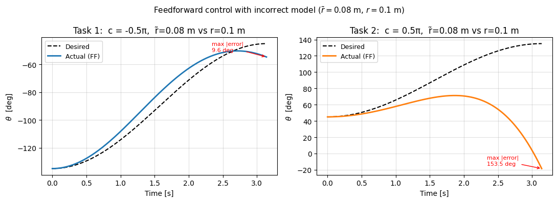
Feedforward + Feedback: Computed Torque Control
For trajectory tracking, the computed torque controller (Eq. 11.35) combines feedforward and PD feedback:
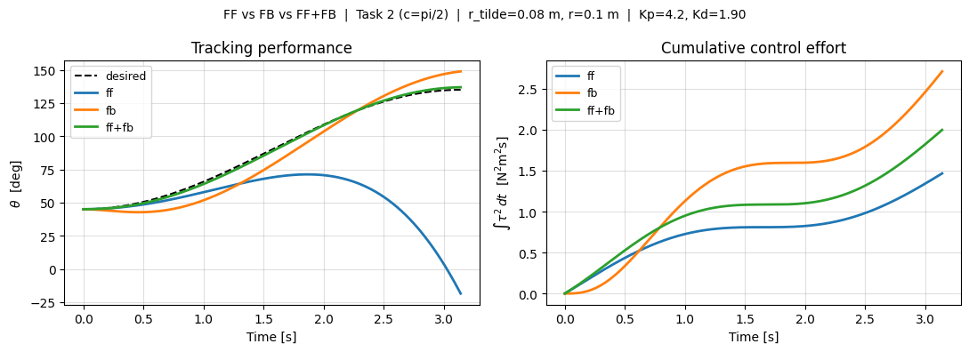
The feedforward term anticipates what torque is needed based on the desired motion and it pre-cancels the known dynamics; the PD feedback corrects residual errors from model mismatch or disturbances. When the model is exact the feedback term is zero. With model mismatch it acts as a corrector, yielding better tracking than either term alone.
Three controllers compared (Task 2 trajectory, ):
| Controller | Torque law | Characteristics |
|---|---|---|
| FF only | Open-loop; large error if model wrong | |
| FB only (PD) | Reactive; some lag/overshoot; high effort | |
| FF+FB (CT) | Sum of above | Best tracking; less effort than FB alone |
The right-hand plot in Fig. 11.19 shows , a standard measure of cumulative control effort.
# =======================================================
# Feedforward + Feedback (Computed Torque) - Fig. 11.19
# =======================================================

# -------------------------------------------------------
# PD gains (design: %OS = 5%, t_settle = 2 s)
# -------------------------------------------------------
percent_OS_fb = 5.0 # percent overshoot
t_settle_fb   = 2.0 # settling time in seconds
ln_os_fb   = np.log(percent_OS_fb / 100.0) # natural log of overshoot
zeta_fb    = -ln_os_fb / np.sqrt(np.pi**2 + ln_os_fb**2) # damping ratio
omega_n_fb = 4.0 / (zeta_fb * t_settle_fb) # natural frequency
Kp_fb = M_link * omega_n_fb**2 # proportional gain
Kd_fb = 2 * zeta_fb * omega_n_fb * M_link - b_link # derivative gain
print(f"PD gains:  Kp = {Kp_fb:.3f} N*m/rad,  Kd = {Kd_fb:.3f} N*m*s/rad")
print(f"           zeta = {zeta_fb:.3f},  omega_n = {omega_n_fb:.3f} rad/s")

# -------------------------------------------------------
# Task 2 desired trajectory  c = pi/2
# -------------------------------------------------------
c_task2 = np.pi / 2

def traj(t, c=None):
    if c is None: c = c_task2
    td   = c - (np.pi / 4) * np.cos(t)
    dtd  =     (np.pi / 4) * np.sin(t)
    ddtd =     (np.pi / 4) * np.cos(t)
    return td, dtd, ddtd

# -------------------------------------------------------
# Three controller torque functions
# -------------------------------------------------------
def tau_ff(t, state):
    td, dtd, ddtd = traj(t)
    h_tilde = m_link * g_acc * r_tilde * np.cos(td) + b_link * dtd
    return M_link * ddtd + h_tilde

def tau_fb(t, state):
    theta, theta_dot = state
    td, dtd, _ = traj(t)
    return Kp_fb * (td - theta) + Kd_fb * (dtd - theta_dot)

def tau_fffb(t, state):
    return tau_ff(t, state) + tau_fb(t, state)

# -------------------------------------------------------
# Simulate all three on the TRUE vertical model
# -------------------------------------------------------
theta0, dtheta0, _ = traj(0.0)
state0 = [theta0, dtheta0]
t_span = (0.0, T_END)

t_ff, th_ff, _       = model_vertical.simulate(tau_ff,   t_span, state0)
t_fb, th_fb, dth_fb  = model_vertical.simulate(tau_fb,   t_span, state0)
t_ct, th_ct, dth_ct  = model_vertical.simulate(tau_fffb, t_span, state0)
th_des = np.array([traj(t)[0] for t in t_ff])

# Torque histories
tau_ff_hist = np.array([tau_ff(t,  [th, dth]) for t, th, dth in zip(t_ff, th_ff, np.gradient(th_ff, t_ff))])
tau_fb_hist = np.array([tau_fb(t,  [th, dth]) for t, th, dth in zip(t_fb, th_fb, dth_fb)])
tau_ct_hist = np.array([tau_fffb(t, [th, dth]) for t, th, dth in zip(t_ct, th_ct, dth_ct)])

# Cumulative control effort: integral of tau^2
def cum_effort(t, tau):
    dt = np.diff(t, prepend=t[0])
    return np.cumsum(tau**2 * dt)

effort_ff = cum_effort(t_ff, tau_ff_hist)
effort_fb = cum_effort(t_fb, tau_fb_hist)
effort_ct = cum_effort(t_ct, tau_ct_hist)

# -------------------------------------------------------
# Figure 1: Tracking + Control Effort (Fig. 11.19)
# -------------------------------------------------------
fig, axes = plt.subplots(1, 2, figsize=(11, 4))

ax = axes[0]
ax.plot(t_ff, np.degrees(th_des), "k--", lw=1.5, label="desired")
ax.plot(t_ff, np.degrees(th_ff),  lw=2, label="ff")
ax.plot(t_fb, np.degrees(th_fb),  lw=2, label="fb")
ax.plot(t_ct, np.degrees(th_ct),  lw=2, label="ff+fb")
ax.set_xlabel("Time [s]")
ax.set_ylabel(r"$\theta$  [deg]")
ax.set_title("Tracking performance")
ax.legend(fontsize=9)
ax.grid(True, alpha=0.4)

ax = axes[1]
ax.plot(t_ff, effort_ff, lw=2, label="ff")
ax.plot(t_fb, effort_fb, lw=2, label="fb")
ax.plot(t_ct, effort_ct, lw=2, label="ff+fb")
ax.set_xlabel("Time [s]")
ax.set_ylabel(r"$\int \tau^2\,dt$  [N$^2$m$^2$s]")
ax.set_title("Cumulative control effort")
ax.legend(fontsize=9)
ax.grid(True, alpha=0.4)

fig.suptitle(
    f"FF vs FB vs FF+FB  |  Task 2 (c=pi/2)  |"
    f"  r_tilde={r_tilde} m, r={r_link} m  |  Kp={Kp_fb:.1f}, Kd={Kd_fb:.2f}",
    fontsize=10,
)
plt.tight_layout()
plt.show()

# =======================================================
# Sinusoidal Trajectory: FF+FB vs FB
# =======================================================
omega_sin = 1.0
A_sin     = np.pi / 4
t_sin_end = 4 * np.pi

def traj_sin(t):
    td   =  A_sin * np.sin(omega_sin * t)
    dtd  =  A_sin * omega_sin * np.cos(omega_sin * t)
    ddtd = -A_sin * omega_sin**2 * np.sin(omega_sin * t)
    return td, dtd, ddtd

def tau_ff_sin(t, state):
    td, dtd, ddtd = traj_sin(t)
    h_tilde = m_link * g_acc * r_tilde * np.cos(td) + b_link * dtd
    return M_link * ddtd + h_tilde

def tau_fb_sin(t, state):
    theta, theta_dot = state
    td, dtd, _ = traj_sin(t)
    return Kp_fb * (td - theta) + Kd_fb * (dtd - theta_dot)

def tau_fffb_sin(t, state):
    return tau_ff_sin(t, state) + tau_fb_sin(t, state)

th0_sin, dth0_sin, _ = traj_sin(0.0)
state0_sin = [th0_sin, dth0_sin]
t_span_sin = (0.0, t_sin_end)

t_s_fb, th_s_fb, dth_s_fb = model_vertical.simulate(tau_fb_sin,   t_span_sin, state0_sin)
t_s_ct, th_s_ct, dth_s_ct = model_vertical.simulate(tau_fffb_sin, t_span_sin, state0_sin)
th_s_des = np.array([traj_sin(t)[0] for t in t_s_fb])

err_fb = np.degrees(th_s_fb - th_s_des)
err_ct = np.degrees(th_s_ct - th_s_des)

fig, axes = plt.subplots(2, 1, figsize=(10, 6), sharex=True)

axes[0].plot(t_s_fb, np.degrees(th_s_des), "k--", lw=1.5, label="desired")
axes[0].plot(t_s_fb, np.degrees(th_s_fb),  lw=2, label="FB (PD)")
axes[0].plot(t_s_ct, np.degrees(th_s_ct),  lw=2, label="FF+FB (CT)")
axes[0].set_ylabel(r"$\theta$  [deg]")
axes[0].set_title(
    r"Sinusoidal tracking: $\theta_d = (\pi/4)\sin(t)$  |  FF+FB vs FB"
)
axes[0].legend(fontsize=9)
axes[0].grid(True, alpha=0.4)

axes[1].plot(t_s_fb, err_fb, lw=2, label="FB error")
axes[1].plot(t_s_ct, err_ct, lw=2, label="FF+FB error")
axes[1].axhline(0, color="gray", linestyle=":", lw=1)
axes[1].fill_between(t_s_fb, err_fb, 0, alpha=0.15)
axes[1].fill_between(t_s_ct, err_ct, 0, alpha=0.15)
axes[1].set_ylabel(r"$\theta_{actual} - \theta_{desired}$  [deg]")
axes[1].set_xlabel("Time [s]")
axes[1].legend(fontsize=9)
axes[1].grid(True, alpha=0.4)

# Mark period boundaries
T_period = 2 * np.pi / omega_sin
for k in range(1, int(t_sin_end / T_period) + 1):
    axes[0].axvline(k * T_period, color="lightgray", lw=0.8, linestyle="--")
    axes[1].axvline(k * T_period, color="lightgray", lw=0.8, linestyle="--")

plt.tight_layout()
plt.show()

rms_fb = np.sqrt(np.mean(err_fb**2))
rms_ct = np.sqrt(np.mean(err_ct**2))
print(f"Sinusoidal tracking RMS error:")
print(f"  FB only : {rms_fb:.3f} deg")
print(f"  FF+FB   : {rms_ct:.3f} deg")
print(f"  Reduction: {(1 - rms_ct/rms_fb)*100:.1f}%")
PD gains:  Kp = 4.199 N*m/rad,  Kd = 1.900 N*m*s/rad
           zeta = 0.690,  omega_n = 2.898 rad/s
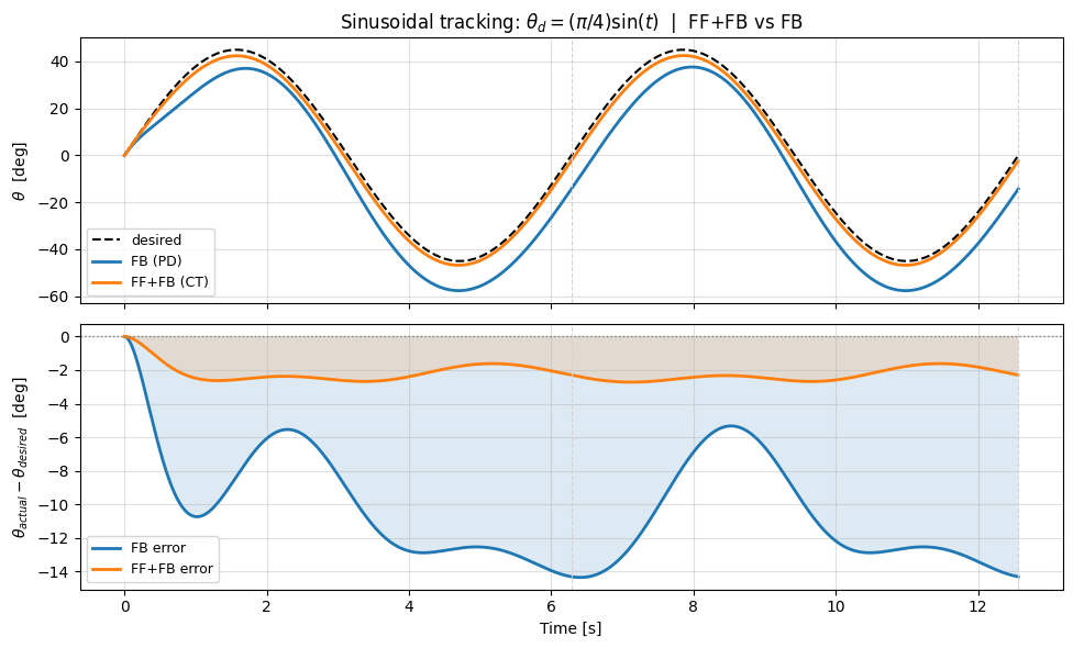
Sinusoidal tracking RMS error:
  FB only : 10.891 deg
  FF+FB   : 2.253 deg
  Reduction: 79.3%
Task 2: Control of a Single Joint Robotic Arm Using MuJoCo
So far the controller and the simulated plant share the same Python model. To better reflect real-world deployment, we now use MuJoCo as the true physical system and the analytical SingleJointModel as the controller’s internal model.
The MuJoCo model is built to match the textbook parameters ( kg m , kg, m, N m s/rad). The controller uses the computed torque law:
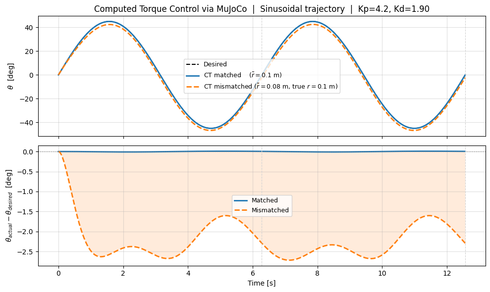
Two scenarios are compared:
| Scenario | Controller model | MuJoCo (true) | Mismatch |
|---|---|---|---|
| Matched | m | m | None — FF cancels dynamics exactly |
| Mismatched | m | m | m — FB must compensate |
This demonstrates that even with an imperfect model, the PD feedback term keeps the system on track — though at the cost of larger control effort than the matched case.
# -------------------------------------------------------
# MuJoCo model: single revolute joint (pendulum)
#
# Parameters match analytical model:
#   joint damping b = 0.1 N*m*s/rad
#   link mass m = 1.0 kg, CoM at r = 0.1 m from joint
#   rotational inertia about joint M = 0.5 kg*m^2
#     -> I_cm_y = M - m*r^2 = 0.5 - 0.01 = 0.49 kg*m^2  (parallel axis)
# -------------------------------------------------------
single_joint_xml = """
<mujoco model="single_joint_arm">
  <option gravity="0 0 -9.81" timestep="0.001"/>
  <worldbody>
    <geom type="sphere" size="0.05" rgba="0.4 0.4 0.4 1"/>
    <body name="link">
      <joint name="j1" type="hinge" axis="0 -1 0" damping="0.1"/>
      <inertial pos="0.1 0 0" mass="1.0" diaginertia="0.001 0.49 0.49"/>
      <geom type="capsule" fromto="0 0 0 0.2 0 0" size="0.02" rgba="0.8 0.3 0.3 1"/>
      <geom type="sphere" pos="0.1 0 0" size="0.025" rgba="0.2 0.6 0.2 1"/>
    </body>
  </worldbody>
  <actuator>
    <motor name="m1" joint="j1" gear="1" ctrlrange="-20 20"/>
  </actuator>
</mujoco>
"""

# -------------------------------------------------------
# Computed torque controller (uses analytical model internally)
# r_ctrl: the CoM distance the CONTROLLER believes (may differ from MuJoCo)
# -------------------------------------------------------
def ct_torque(t, theta, theta_dot, traj_func, r_ctrl):
    td, dtd, ddtd = traj_func(t)
    # Feedforward using controller model
    h_ctrl = m_link * g_acc * r_ctrl * np.cos(td) + b_link * dtd
    tau_ff_val = M_link * ddtd + h_ctrl
    # PD feedback on tracking error
    tau_fb_val = Kp_fb * (td - theta) + Kd_fb * (dtd - theta_dot)
    return tau_ff_val + tau_fb_val

# -------------------------------------------------------
# MuJoCo simulation loop
# -------------------------------------------------------
def run_mujoco(traj_func, r_ctrl, duration, tau_limit=20.0):
    mj_m = mujoco.MjModel.from_xml_string(single_joint_xml)
    mj_d = mujoco.MjData(mj_m)
    # Set initial conditions to match trajectory start
    th0, dth0, _ = traj_func(0.0)
    mj_d.qpos[0] = th0
    mj_d.qvel[0] = dth0
    mujoco.mj_forward(mj_m, mj_d)

    times, thetas, theta_dots, taus = [], [], [], []
    while mj_d.time < duration:
        t      = mj_d.time
        theta  = mj_d.qpos[0]
        thetad = mj_d.qvel[0]
        tau    = ct_torque(t, theta, thetad, traj_func, r_ctrl)
        tau    = float(np.clip(tau, -tau_limit, tau_limit)) # clip torque to actuator limits
        mj_d.ctrl[0] = tau # apply computed torque to MuJoCo actuator
        times.append(t)
        thetas.append(theta)
        theta_dots.append(thetad)
        taus.append(tau)
        mujoco.mj_step(mj_m, mj_d) # advance MuJoCo simulation by one timestep

    return (np.array(times), np.array(thetas),
            np.array(theta_dots), np.array(taus))

# -------------------------------------------------------
# Simulate: sinusoidal trajectory, two mismatch scenarios
# -------------------------------------------------------
duration_mj = t_sin_end   # reuse sinusoidal trajectory from above

print("Running MuJoCo simulation - matched model (r_ctrl = 0.1)...")
t_match, th_match, _, tau_match = run_mujoco(traj_sin, r_ctrl=r_link,   duration=duration_mj)
print("Running MuJoCo simulation - mismatched model (r_ctrl = 0.08)...")
t_mis,   th_mis,   _, tau_mis   = run_mujoco(traj_sin, r_ctrl=r_tilde,  duration=duration_mj)
print("Done.")

# Desired trajectory sampled at MuJoCo timesteps
th_des_mj   = np.array([traj_sin(t)[0] for t in t_match])
err_match   = np.degrees(th_match - th_des_mj)
err_mis     = np.degrees(th_mis   - np.array([traj_sin(t)[0] for t in t_mis]))

# -------------------------------------------------------
# Figure 1: Trajectory tracking
# -------------------------------------------------------
fig, axes = plt.subplots(2, 1, figsize=(10, 6), sharex=True)

axes[0].plot(t_match, np.degrees(th_des_mj), "k--", lw=1.5, label="Desired")
axes[0].plot(t_match, np.degrees(th_match),  lw=2,  label=f"CT matched    ($\\tilde{{r}}={r_link}$ m)")
axes[0].plot(t_mis,   np.degrees(th_mis),    lw=2,  linestyle="--",
             label=f"CT mismatched ($\\tilde{{r}}={r_tilde}$ m, true $r={r_link}$ m)")
axes[0].set_ylabel(r"$\theta$  [deg]")
axes[0].set_title(
    f"Computed Torque Control via MuJoCo  |  "
    f"Sinusoidal trajectory  |  Kp={Kp_fb:.1f}, Kd={Kd_fb:.2f}"
)
axes[0].legend(fontsize=9)
axes[0].grid(True, alpha=0.4)

axes[1].plot(t_match, err_match, lw=2, label="Matched")
axes[1].plot(t_mis,   err_mis,   lw=2, linestyle="--", label="Mismatched")
axes[1].axhline(0, color="gray", linestyle=":", lw=1)
axes[1].fill_between(t_match, err_match, 0, alpha=0.15)
axes[1].fill_between(t_mis,   err_mis,   0, alpha=0.15)
axes[1].set_ylabel(r"$\theta_{actual} - \theta_{desired}$  [deg]")
axes[1].set_xlabel("Time [s]")
axes[1].legend(fontsize=9)
axes[1].grid(True, alpha=0.4)

T_period_mj = 2 * np.pi / omega_sin
for k in range(1, int(duration_mj / T_period_mj) + 1):
    axes[0].axvline(k * T_period_mj, color="lightgray", lw=0.8, linestyle="--")
    axes[1].axvline(k * T_period_mj, color="lightgray", lw=0.8, linestyle="--")

plt.tight_layout()
plt.show()

# -------------------------------------------------------
# Figure 2: Torque comparison
# -------------------------------------------------------
effort_match = np.cumsum(tau_match**2 * np.diff(t_match, prepend=t_match[0]))
effort_mis   = np.cumsum(tau_mis**2   * np.diff(t_mis,   prepend=t_mis[0]))

fig, axes = plt.subplots(1, 2, figsize=(11, 3.5))

axes[0].plot(t_match, tau_match, lw=2, label="Matched")
axes[0].plot(t_mis,   tau_mis,   lw=2, linestyle="--", label="Mismatched")
axes[0].axhline(0, color="gray", linestyle=":", lw=1)
axes[0].set_ylabel(r"$\tau$  [N$\cdot$m]")
axes[0].set_xlabel("Time [s]")
axes[0].set_title("Applied torque")
axes[0].legend(fontsize=9)
axes[0].grid(True, alpha=0.4)

axes[1].plot(t_match, effort_match, lw=2, label="Matched")
axes[1].plot(t_mis,   effort_mis,   lw=2, linestyle="--", label="Mismatched")
axes[1].set_ylabel(r"$\int\tau^2\,dt$  [N$^2$m$^2$s]")
axes[1].set_xlabel("Time [s]")
axes[1].set_title("Cumulative control effort")
axes[1].legend(fontsize=9)
axes[1].grid(True, alpha=0.4)

plt.tight_layout()
plt.show()

# Summary
rms_match = np.sqrt(np.mean(err_match**2))
rms_mis   = np.sqrt(np.mean(err_mis**2))
print(f"MuJoCo CT control RMS tracking error:")
print(f"  Matched model    (r_ctrl={r_link}):   {rms_match:.4f} deg")
print(f"  Mismatched model (r_ctrl={r_tilde}): {rms_mis:.4f} deg")
print(f"  Mismatch penalty: {rms_mis - rms_match:.4f} deg  "
      f"(FB compensates {(1-rms_mis/rms_match)*100 if rms_mis < rms_match else 0:.0f}%)")
Running MuJoCo simulation - matched model (r_ctrl = 0.1)...
Running MuJoCo simulation - mismatched model (r_ctrl = 0.08)...
Done.
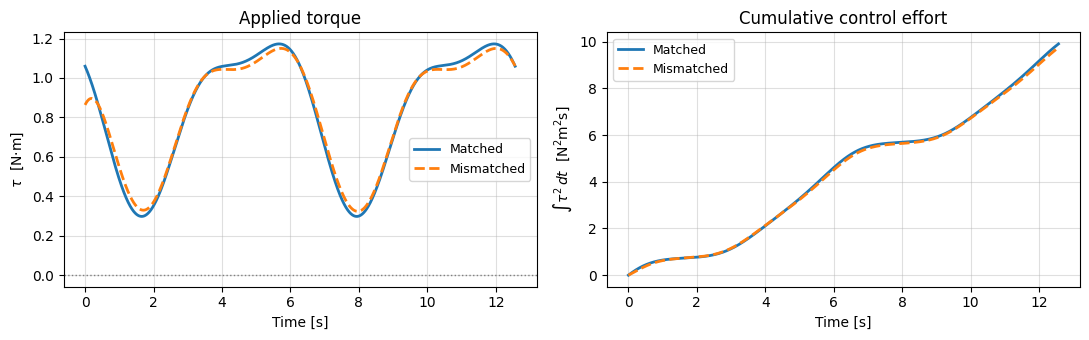
MuJoCo CT control RMS tracking error:
  Matched model    (r_ctrl=0.1):   0.0069 deg
  Mismatched model (r_ctrl=0.08): 2.2551 deg
  Mismatch penalty: 2.2481 deg  (FB compensates 0%)
Task 3: Control of a 2R Planar Robot Using MuJoCo
In Tasks 1 and 2, we designed and verified computed torque control for a single-joint arm. Here we extend the approach to a 2R planar robot, and use MuJoCo as the plant for both simulation and dynamics extraction.
Dynamics
The joint-space equations of motion are:
where are the joint angles, is the inertia matrix, and collects Coriolis and centrifugal terms. Gravity is disabled in this horizontal planar setup.
MuJoCo exposes these terms directly:
mujoco.mj_crba(model, data)runs the Composite Rigid-Body Algorithm (CRBA) at the current joint configurationdata.qposto assemble the joint-space inertia in MuJoCo’s internal sparse format (data.qM).mujoco.mj_fullM(model, M_full, data.qM)converts that internal representation into a dense matrixM_full, giving the explicit inertia matrix used in computed-torque control.data.qfrc_biasis MuJoCo’s bias-force vector evaluated at the current state (q,\dot q), containing velocity-dependent terms (Coriolis/centrifugal) and gravity contributions; with gravity disabled, it mainly represents .
We first create the MuJoCo model.
import os
import mujoco
import numpy as np
import matplotlib
matplotlib.use("Agg")
import matplotlib.pyplot as plt
import matplotlib.animation as animation
from IPython.display import HTML, display

# ── Robot parameters (matching Task 4) ────────────────────────────────────────
m1, m2 = 1.0, 0.8      # link masses [kg]
l1, l2 = 0.5, 0.4      # link lengths [m]

# Inertia of each link as a uniform rod, about COM: I = m*L^2/12
I1_zz = m1 * l1**2 / 12
I2_zz = m2 * l2**2 / 12

# ── Step 1: Create the MuJoCo XML ─────────────────────────────────────────────
# - Robot in the XY plane, joints rotate about Z-axis
# - You can assign gravity to either enable or disable gravity term in EOM
# - <inertial> tags set exact uniform-rod inertia to match the analytical model
xml_content = f"""<mujoco model="2r_planar_robot">
  <option gravity="0 0 0" timestep="0.002" integrator="RK4"/>
  <compiler balanceinertia="true"/>

  <default>
    <joint damping="0" frictionloss="0"/>
    <motor ctrllimited="false"/>
  </default>

  <worldbody>
    <camera name="xy_plane" pos="0 0 2" euler="0 0 0" fovy="60"/>
    <light pos="0 0 3" dir="0 0 -1"/>

    <!-- Link 1: hinge at origin, uniform-rod inertia about COM -->
    <body name="link1" pos="0 0 0">
      <joint name="joint1" type="hinge" axis="0 0 1"/>
      <! We set Ixx = Iyy = I_zz/2 so that it satisfies MuJoCo's triangle inequality (A + B ≥ C)>
      <!Only Izz actually affects the dynamics. Ixx and Iyy are never "activated" in this planar setup>
      <!they're just dummy values chosen to satisfy MuJoCo's requirement.>
      <inertial pos="{l1/2:.4f} 0 0" mass="{m1}"
                diaginertia="{I1_zz/2:.6f} {I1_zz/2:.6f} {I1_zz:.6f}"/>
      <geom type="capsule" fromto="0 0 0 {l1} 0 0" size="0.025"
            rgba="0.2 0.6 0.9 1" mass="0"/>

      <!-- Link 2: hinge at end of link1 -->
      <body name="link2" pos="{l1} 0 0">
        <joint name="joint2" type="hinge" axis="0 0 1"/>
        <inertial pos="{l2/2:.4f} 0 0" mass="{m2}"
                  diaginertia="{I2_zz/2:.6f} {I2_zz/2:.6f} {I2_zz:.6f}"/>
        <geom type="capsule" fromto="0 0 0 {l2} 0 0" size="0.02"
              rgba="0.9 0.4 0.2 1" mass="0"/>
        <site name="end_effector" pos="{l2} 0 0" size="0.03" rgba="1 0 0 1"/>
      </body>
    </body>
  </worldbody>

  <actuator>
    <motor name="tau1" joint="joint1"/>
    <motor name="tau2" joint="joint2"/>
  </actuator>
</mujoco>"""

xml_path = "2r_robot.xml"
with open(xml_path, "w") as f:
    f.write(xml_content)
print(f"XML saved: {xml_path}")

# ── Step 2: Load MuJoCo model ──────────────────────────────────────────────────
model = mujoco.MjModel.from_xml_path(xml_path)
data  = mujoco.MjData(model)
XML saved: 2r_robot.xml
Task 3.1: Reaching Task
Goal: Drive the end-effector to a random reachable target point from an arbitrary initial configuration. We will use the PD controller and the computed torque controller.
PD Feedback Controller without Feedforward -- Joint Space
We can achieve this using a PD controller.
where and . Note that is a two-dimensional vector.
Computed Torque Control -- Joint Space
For set-point control (reaching a target joint configuration ):
With a constant target (), the bias term cancels and the closed-loop error dynamics decouple into two independent second-order systems:
Approach:
Sample a random target inside the reachable workspace (annulus: )
Solve analytical inverse kinematics (IK) to obtain the desired joint angles
Apply joint-space PD controller or computed torque controller to drive
Inverse Kinematics (2R planar, elbow-up):
Gain design: Choosing natural frequency and damping ratio for the error dynamics :
These values are chosen to match the standard second-order form
So, directly sets response speed (larger faster convergence), and sets damping/overshoot ( gives fast, well-damped motion with little overshoot).
# -----------------------------------------------------------------------
# Task 3.1: Reaching Task - PD vs Computed Torque Control (Joint Space)
# -----------------------------------------------------------------------

# ---- Helper functions --------------------------------------------------

def fk_2r(q, l1, l2):
    """Forward kinematics: joint angles -> end-effector (x, y)."""
    x = l1 * np.cos(q[0]) + l2 * np.cos(q[0] + q[1])
    y = l1 * np.sin(q[0]) + l2 * np.sin(q[0] + q[1])
    return np.array([x, y])

def jacobian_2r(q, l1, l2):
    """2x2 geometric Jacobian of the 2R planar robot."""
    s1  = np.sin(q[0]);        c1  = np.cos(q[0])
    s12 = np.sin(q[0]+q[1]);   c12 = np.cos(q[0]+q[1])
    return np.array([
        [-l1*s1 - l2*s12,  -l2*s12],
        [ l1*c1 + l2*c12,   l2*c12]
    ])

def jdot_qdot_2r(q, qd, l1, l2):
    """Jdot @ qdot: centripetal acceleration term for 2R robot."""
    c1  = np.cos(q[0]);        s1  = np.sin(q[0])
    c12 = np.cos(q[0]+q[1]);   s12 = np.sin(q[0]+q[1])
    q1d, q12d = qd[0], qd[0] + qd[1]
    ax = -l1*c1*q1d**2 - l2*c12*q12d**2
    ay = -l1*s1*q1d**2 - l2*s12*q12d**2
    return np.array([ax, ay])

def ik_2r(px, py, l1, l2, elbow_up=True):
    """Analytical IK for 2R planar robot (elbow-up or elbow-down)."""
    D = (px**2 + py**2 - l1**2 - l2**2) / (2.0 * l1 * l2)
    D = np.clip(D, -1.0, 1.0)
    q2 = np.arccos(D) if elbow_up else -np.arccos(D)
    q1 = np.arctan2(py, px) - np.arctan2(l2*np.sin(q2), l1 + l2*np.cos(q2))
    return np.array([q1, q2])

def get_mass_matrix(model, data):
    """Extract the full mass matrix M(q) from MuJoCo."""
    M_full = np.zeros((model.nv, model.nv))  # initialize mass matrix
    mujoco.mj_fullM(model, M_full, data.qM) # compute the full inertia matrix
    return M_full

def pd_joint_torque(data, q_d, Kp, Kd):
    """Simple joint-space PD: tau = Kp*(q_d - q) + Kd*(0 - qdot).
    No model knowledge -- treats each joint independently.
    """
    e  =  q_d - data.qpos
    ed = -data.qvel          # desired velocity = 0 for set-point
    return Kp * e + Kd * ed

def ct_joint_torque(model, data, q_d, Kp, Kd):
    """Computed torque: tau = M(q)*(Kp*e + Kd*ed) + bias.
    Cancels inertia coupling and Coriolis -- decoupled linear error dynamics.
    """
    e  =  q_d - data.qpos
    ed = -data.qvel
    M    = get_mass_matrix(model, data)
    bias = data.qfrc_bias.copy()  # Coriolis, centrifugal, and gravity terms
    return M @ (Kp * e + Kd * ed) + bias

# ---- Random reachable target -------------------------------------------
rng   = np.random.default_rng(seed=42)
r_min = abs(l1 - l2) + 0.05  # minimum reachable radius
r_max = l1 + l2 - 0.05       # maximum reachable radius

r_tgt     = rng.uniform(r_min, r_max)  # random target radius
th_tgt    = rng.uniform(-np.pi, np.pi)  # random target angle
target_xy = r_tgt * np.array([np.cos(th_tgt), np.sin(th_tgt)])  # target position in XY
q_des     = ik_2r(target_xy[0], target_xy[1], l1, l2, elbow_up=True)  # desired joint angles
q0        = np.array([0.2, 0.3])   # shared initial configuration, you may change this

print(f'Target:        ({target_xy[0]:.3f}, {target_xy[1]:.3f}) m')
print(f'Desired joints: q1={np.degrees(q_des[0]):.1f} deg,  q2={np.degrees(q_des[1]):.1f} deg')

# ---- Controller gains -------------------------------------------------
# CT: gains directly set error dynamics wn = sqrt(Kp), zeta = Kd/(2*wn)
#     because M(q) is fully cancelled -> decoupled linear response.
wn_ct   = 10.0
zeta_ct = 0.9
Kp_ct   = wn_ct**2               # 100
Kd_ct   = 2 * zeta_ct * wn_ct   # 18

# PD: no inertia cancellation -> effective wn_eff = sqrt(Kp/M_eff).
#     Needs higher Kp to drive the same convergence speed against the
#     actual inertia (M_eff ~ 0.3 kg*m^2 for joint 1, ~0.04 for joint 2).
Kp_pd   = 40
Kd_pd   = 1

# ---- Simulation helper ------------------------------------------------
def run_sim(ctrl_fn):
    mujoco.mj_resetData(model, data)
    data.qpos[:] = q0
    data.qvel[:] = [0.0, 0.0]
    mujoco.mj_forward(model, data)
    n  = int(T_sim / model.opt.timestep)
    tl = np.zeros(n);  ql = np.zeros((n, 2))
    tl2 = np.zeros((n, 2));  el = np.zeros((n, 2))

    for k in range(n):
        tau = ctrl_fn()
        data.ctrl[:] = tau
        mujoco.mj_step(model, data)
        tl[k]  = data.time
        ql[k]  = data.qpos.copy()
        tl2[k] = tau
        el[k]  = fk_2r(data.qpos, l1, l2)
    return tl, ql, tl2, el

T_sim = 3.0

#conduct simulation for PD controller
t_pd,  q_pd,  tau_pd,  ee_pd  = run_sim(
    lambda: pd_joint_torque(data, q_des, Kp_pd, Kd_pd))

#conduct simulation for CT controller
t_ct,  q_ct,  tau_ct,  ee_ct  = run_sim(
    lambda: ct_joint_torque(model, data, q_des, Kp_ct, Kd_ct))

# ---- Static comparison plots ------------------------------------------
fig, axes = plt.subplots(2, 3, figsize=(15, 8))
fig.suptitle('Task 3.1: Reaching Task - PD vs Computed Torque Control', fontsize=13)

# --- Joint angle errors
for j, (ax, joint, col) in enumerate(zip(axes[0, :2],
                                          ['Joint 1', 'Joint 2'],
                                          [0, 1])):
    ax.plot(t_pd, np.degrees(q_pd[:, col] - q_des[col]), 'C1', label='PD')
    ax.plot(t_ct, np.degrees(q_ct[:, col] - q_des[col]), 'C0', label='CT')
    ax.axhline(0, color='k', lw=0.8, ls='--')
    ax.set_xlabel('Time [s]'); ax.set_ylabel('Error [deg]')
    ax.set_title(f'{joint} Error'); ax.legend(); ax.grid(True)

# --- EE path in XY
ax = axes[0, 2]
ax.set_aspect('equal')
theta_ws = np.linspace(0, 2*np.pi, 300)
ax.plot((l1+l2)*np.cos(theta_ws), (l1+l2)*np.sin(theta_ws), 'k--', alpha=0.15, lw=1)
ax.plot(r_min*np.cos(theta_ws),   r_min*np.sin(theta_ws),   'k--', alpha=0.15, lw=1)
ax.plot(ee_pd[:, 0], ee_pd[:, 1], 'C1-', lw=1.5, label='PD')
ax.plot(ee_ct[:, 0], ee_ct[:, 1], 'C0-', lw=1.5, label='CT')
ax.plot(ee_pd[0, 0], ee_pd[0, 1], 'go', ms=9, label='Start')
ax.plot(*target_xy, 'r*', ms=14, zorder=5, label='Target')
ax.set_xlabel('X [m]'); ax.set_ylabel('Y [m]')
ax.set_title('End-Effector Path'); ax.legend(fontsize=8); ax.grid(True)

# --- Control torques
for j, (ax, joint, col) in enumerate(zip(axes[1, :2],
                                          ['tau1', 'tau2'],
                                          [0, 1])):
    ax.plot(t_pd, tau_pd[:, col], 'C1', label='PD')
    ax.plot(t_ct, tau_ct[:, col], 'C0', label='CT')
    ax.set_xlabel('Time [s]'); ax.set_ylabel('Torque [N m]')
    ax.set_title(f'{joint}'); ax.legend(); ax.grid(True)

# --- EE distance to target over time
ax = axes[1, 2]
dist_pd = np.linalg.norm(ee_pd - target_xy, axis=1) * 1000
dist_ct = np.linalg.norm(ee_ct - target_xy, axis=1) * 1000
ax.plot(t_pd, dist_pd, 'C1', label='PD')
ax.plot(t_ct, dist_ct, 'C0', label='CT')
ax.set_xlabel('Time [s]'); ax.set_ylabel('Distance [mm]')
ax.set_title('EE Distance to Target'); ax.legend(); ax.grid(True)

plt.tight_layout()
display(fig)
plt.close(fig)

print(f'Final EE error -- PD: {dist_pd[-1]:.2f} mm   CT: {dist_ct[-1]:.2f} mm')


# ---- Animation: both arms side by side --------------------------------
from matplotlib.animation import FuncAnimation

stride = max(1, len(t_pd) // 150)
q_pd_s  = q_pd[::stride];  ee_pd_s = ee_pd[::stride]
q_ct_s  = q_ct[::stride];  ee_ct_s = ee_ct[::stride]
n_frames = len(q_pd_s)

fig_a, (axL, axR) = plt.subplots(1, 2, figsize=(12, 6))
fig_a.suptitle('Task 3.1: PD (left) vs Computed Torque (right)', fontsize=12)
R = l1 + l2 + 0.1

for ax, title in zip([axL, axR], ['PD Control', 'Computed Torque Control']):
    ax.set_xlim(-R, R); ax.set_ylim(-R, R)
    ax.set_aspect('equal'); ax.grid(True)
    ax.set_title(title)
    ax.plot((l1+l2)*np.cos(theta_ws), (l1+l2)*np.sin(theta_ws), 'k--', alpha=0.15, lw=1)
    ax.plot(r_min*np.cos(theta_ws),   r_min*np.sin(theta_ws),   'k--', alpha=0.15, lw=1)
    ax.plot(*target_xy, 'r*', ms=14, zorder=5)

arm_pd,   = axL.plot([], [], 'o-', lw=3, color='C1', ms=6)
trace_pd, = axL.plot([], [], '-',  lw=1.5, color='C1', alpha=0.5)
arm_ct,   = axR.plot([], [], 'o-', lw=3, color='C0', ms=6)
trace_ct, = axR.plot([], [], '-',  lw=1.5, color='C0', alpha=0.5)

def _arm_pts(q):
    elbow = np.array([l1*np.cos(q[0]), l1*np.sin(q[0])])
    ee    = fk_2r(q, l1, l2)
    return [0, elbow[0], ee[0]], [0, elbow[1], ee[1]]

def _init_a():
    for ln in [arm_pd, trace_pd, arm_ct, trace_ct]:
        ln.set_data([], [])
    return arm_pd, trace_pd, arm_ct, trace_ct

def _update_a(i):
    xs, ys = _arm_pts(q_pd_s[i])
    arm_pd.set_data(xs, ys)
    trace_pd.set_data(ee_pd_s[:i+1, 0], ee_pd_s[:i+1, 1])
    xs, ys = _arm_pts(q_ct_s[i])
    arm_ct.set_data(xs, ys)
    trace_ct.set_data(ee_ct_s[:i+1, 0], ee_ct_s[:i+1, 1])
    return arm_pd, trace_pd, arm_ct, trace_ct

ani_a = FuncAnimation(fig_a, _update_a, frames=n_frames,
                      init_func=_init_a, interval=20, blit=True)
plt.close(fig_a)
display(HTML(ani_a.to_jshtml()))
Output hidden; open in https://colab.research.google.com to view.Task 3.2: Trajectory Tracking
Goal: Track a circular Cartesian trajectory in the XY plane.
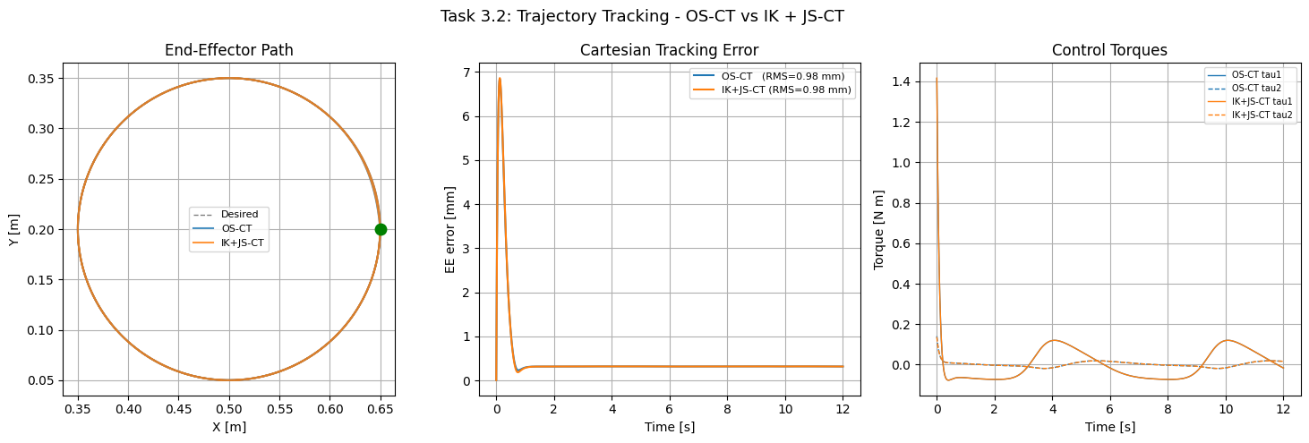
We implement and compare two approaches:
Method A — Operational-Space Computed Torque (OS-CT)
Control the Cartesian error directly, without converting to joint space:
where is the Cartesian error, is the Cartesian velocity error, and is the centripetal acceleration term.
Method B — IK + Joint-Space Computed Torque (IK + JS-CT)
First convert the Cartesian trajectory into a joint trajectory at every timestep, then apply the same joint-space CT controller used in Task 3.1:
Desired joint angles via inverse kinematics:
Desired joint velocities via Jacobian inverse:
Desired joint accelerations with centripetal correction:
Joint-space CT (same law as Task 3.1, now with feedforward):
Both methods share the same gains (, ) and produce theoretically equivalent error dynamics. Differences in practice arise from the IK branch’s sensitivity near joint singularities and discretization of the Jacobian.
# -----------------------------------------------------------------------
# Task 3.2: Trajectory Tracking
#   Method A: Operational-Space Computed Torque
#   Method B: IK + Joint-Space Computed Torque
# -----------------------------------------------------------------------

# ---- Desired circular trajectory --------------------------------------
center  = np.array([0.5, 0.2])
radius  = 0.15
omega_c = 2 * np.pi / 6.0   # one circle per 6 s

def desired_trajectory(t):
    """Desired circular position, velocity, and acceleration."""
    x_d   = center + radius * np.array([ np.cos(omega_c*t),  np.sin(omega_c*t)])
    xd_d  = radius * omega_c * np.array([-np.sin(omega_c*t),  np.cos(omega_c*t)])
    xdd_d = radius * omega_c**2 * np.array([-np.cos(omega_c*t), -np.sin(omega_c*t)])
    return x_d, xd_d, xdd_d

# ---- Controller A: Operational-Space CT --------------------------------
def ct_op_torque(model, data, x_d, xd_d, xdd_d, Kp, Kd):
    """
    Operational-space CT:
      tau = M(q) J^{-1}(xdd_d + Kd*ex_d + Kp*ex - Jdot*qdot) + bias
    Controls Cartesian error directly without IK.
    """
    q, qd = data.qpos.copy(), data.qvel.copy()
    J    = jacobian_2r(q, l1, l2)
    ex   = x_d  - fk_2r(q, l1, l2)
    exd  = xd_d - J @ qd
    Jdqd = jdot_qdot_2r(q, qd, l1, l2)
    M    = get_mass_matrix(model, data)
    bias = data.qfrc_bias.copy()
    v    = xdd_d + Kd * exd + Kp * ex - Jdqd
    return M @ np.linalg.solve(J, v) + bias

# ---- Controller B: IK + Joint-Space CT ---------------------------------
def ct_ik_joint_torque(model, data, x_d, xd_d, xdd_d, Kp, Kd):
    """
    IK + Joint-Space CT (extends ct_joint_torque from Task 3.1):
      Step 1 - Convert Cartesian trajectory to joint trajectory via IK:
        q_d   = IK(x_d)                         (desired joint angles)
        qd_d  = J(q_d)^{-1} * xd_d              (desired joint velocities)
        qdd_d = J(q_d)^{-1} * (xdd_d - Jdot*qd_d) (desired joint accelerations)
      Step 2 - Apply joint-space CT with feedforward:
        tau = M(q)(qdd_d + Kd*(qd_d - qdot) + Kp*(q_d - q)) + bias
    """
    q, qd = data.qpos.copy(), data.qvel.copy()

    # Step 1: Cartesian -> joint trajectory
    q_d  = ik_2r(x_d[0], x_d[1], l1, l2, elbow_up=True)
    J_d  = jacobian_2r(q_d, l1, l2)
    qd_d = np.linalg.solve(J_d, xd_d) # desired joint velocities via IK, this is obtained by inverting the Jacobian
    Jdqd = jdot_qdot_2r(q_d, qd_d, l1, l2)
    qdd_d = np.linalg.solve(J_d, xdd_d - Jdqd) # desired joint accelerations via IK

    # Step 2: Joint-space CT (same structure as ct_joint_torque in Task 3.1,
    #         extended with feedforward acceleration qdd_d)
    e  = q_d  - q
    ed = qd_d - qd
    M    = get_mass_matrix(model, data)
    bias = data.qfrc_bias.copy()
    return M @ (qdd_d + Kd * ed + Kp * e) + bias

# ---- Shared gains and initial condition --------------------------------
# Both controllers use the same wn=8, zeta=1.0 for a fair comparison
wn_t   = 8.0
zeta_t = 1.0
Kp_t   = wn_t**2             # 64
Kd_t   = 2 * zeta_t * wn_t  # 16

x0_traj, _, _ = desired_trajectory(0.0)
q0_traj = ik_2r(x0_traj[0], x0_traj[1], l1, l2, elbow_up=True)
T_traj  = 12.0   # two full circles
dt      = model.opt.timestep
n_steps = int(T_traj / dt)

# ---- Simulation helper ------------------------------------------------
def run_tracking(ctrl_fn):
    mujoco.mj_resetData(model, data)
    data.qpos[:] = q0_traj
    data.qvel[:] = [0.0, 0.0]
    mujoco.mj_forward(model, data)
    t_l  = np.zeros(n_steps)
    ee_l = np.zeros((n_steps, 2))
    xd_l = np.zeros((n_steps, 2))
    xe_l = np.zeros((n_steps, 2))
    tau_l = np.zeros((n_steps, 2))
    q_l  = np.zeros((n_steps, 2))
    for k in range(n_steps):
        t_now = data.time
        x_d, xd_d, xdd_d = desired_trajectory(t_now)
        tau = ctrl_fn(x_d, xd_d, xdd_d)
        data.ctrl[:] = tau
        mujoco.mj_step(model, data)
        t_l[k]   = data.time
        q_l[k]   = data.qpos.copy()
        ee_l[k]  = fk_2r(data.qpos, l1, l2)
        xd_l[k]  = x_d
        xe_l[k]  = x_d - fk_2r(data.qpos, l1, l2)
        tau_l[k] = tau
    return t_l, q_l, ee_l, xd_l, xe_l, tau_l

print('Running OS-CT simulation...')
t_os, q_os, ee_os, xd_os, xe_os, tau_os = run_tracking(
    lambda x_d, xd_d, xdd_d: ct_op_torque(model, data, x_d, xd_d, xdd_d, Kp_t, Kd_t))

print('Running IK + JS-CT simulation...')
t_ik, q_ik, ee_ik, xd_ik, xe_ik, tau_ik = run_tracking(
    lambda x_d, xd_d, xdd_d: ct_ik_joint_torque(model, data, x_d, xd_d, xdd_d, Kp_t, Kd_t))

rms_os = np.sqrt(np.mean(xe_os**2, axis=0)) * 1000
rms_ik = np.sqrt(np.mean(xe_ik**2, axis=0)) * 1000
print(f'RMS error -- OS-CT:    ex={rms_os[0]:.3f} mm, ey={rms_os[1]:.3f} mm')
print(f'RMS error -- IK+JS-CT: ex={rms_ik[0]:.3f} mm, ey={rms_ik[1]:.3f} mm')

# ---- Comparison plots -------------------------------------------------
theta_c  = np.linspace(0, 2*np.pi, 300)
circle_x = center[0] + radius * np.cos(theta_c)
circle_y = center[1] + radius * np.sin(theta_c)

fig, axes = plt.subplots(1, 3, figsize=(15, 5))
fig.suptitle('Task 3.2: Trajectory Tracking - OS-CT vs IK + JS-CT', fontsize=13)

ax = axes[0]
ax.set_aspect('equal')
ax.plot(circle_x, circle_y, 'k--', lw=1, alpha=0.5, label='Desired')
ax.plot(ee_os[:, 0], ee_os[:, 1], 'C0-', lw=1.5, alpha=0.8, label='OS-CT')
ax.plot(ee_ik[:, 0], ee_ik[:, 1], 'C1-', lw=1.5, alpha=0.8, label='IK+JS-CT')
ax.plot(ee_os[0, 0], ee_os[0, 1], 'go', ms=9)
ax.set_xlabel('X [m]'); ax.set_ylabel('Y [m]')
ax.set_title('End-Effector Path'); ax.legend(fontsize=8); ax.grid(True)

ax = axes[1]
err_os = np.linalg.norm(xe_os, axis=1) * 1000
err_ik = np.linalg.norm(xe_ik, axis=1) * 1000
ax.plot(t_os, err_os, 'C0', label=f'OS-CT   (RMS={np.sqrt(np.mean(err_os**2)):.2f} mm)')
ax.plot(t_ik, err_ik, 'C1', label=f'IK+JS-CT (RMS={np.sqrt(np.mean(err_ik**2)):.2f} mm)')
ax.set_xlabel('Time [s]'); ax.set_ylabel('EE error [mm]')
ax.set_title('Cartesian Tracking Error'); ax.legend(fontsize=8); ax.grid(True)

ax = axes[2]
ax.plot(t_os, tau_os[:, 0], 'C0-',  lw=1,   label='OS-CT tau1')
ax.plot(t_os, tau_os[:, 1], 'C0--', lw=1,   label='OS-CT tau2')
ax.plot(t_ik, tau_ik[:, 0], 'C1-',  lw=1,   label='IK+JS-CT tau1')
ax.plot(t_ik, tau_ik[:, 1], 'C1--', lw=1,   label='IK+JS-CT tau2')
ax.set_xlabel('Time [s]'); ax.set_ylabel('Torque [N m]')
ax.set_title('Control Torques'); ax.legend(fontsize=7); ax.grid(True)

plt.tight_layout()
display(fig)
plt.close(fig)

# ---- Side-by-side animation -------------------------------------------
from matplotlib.animation import FuncAnimation

stride = max(1, n_steps // 300)
q_os_s  = q_os[::stride];  ee_os_s = ee_os[::stride];  xd_s = xd_os[::stride]
q_ik_s  = q_ik[::stride];  ee_ik_s = ee_ik[::stride]
n_fr    = len(q_os_s)

fig_a, (axL, axR) = plt.subplots(1, 2, figsize=(12, 6))
fig_a.suptitle('Task 3.2: OS-CT (left) vs IK + JS-CT (right)', fontsize=12)
R2 = l1 + l2 + 0.1

for ax, title in zip([axL, axR],
                     ['Operational-Space CT', 'IK + Joint-Space CT']):
    ax.set_xlim(-R2, R2); ax.set_ylim(-R2, R2)
    ax.set_aspect('equal'); ax.grid(True); ax.set_title(title)
    ax.plot(circle_x, circle_y, 'k--', lw=1, alpha=0.3)

arm_os,   = axL.plot([], [], 'o-', lw=3, color='C0', ms=6)
trace_os, = axL.plot([], [], '-',  lw=1.5, color='C0', alpha=0.5)
des_os,   = axL.plot([], [], 'r*', ms=10, zorder=5)
arm_ik,   = axR.plot([], [], 'o-', lw=3, color='C1', ms=6)
trace_ik, = axR.plot([], [], '-',  lw=1.5, color='C1', alpha=0.5)
des_ik,   = axR.plot([], [], 'r*', ms=10, zorder=5)

def _arm(q):
    elbow = np.array([l1*np.cos(q[0]), l1*np.sin(q[0])])
    ee    = fk_2r(q, l1, l2)
    return [0, elbow[0], ee[0]], [0, elbow[1], ee[1]]

def _init_a():
    for ln in [arm_os, trace_os, des_os, arm_ik, trace_ik, des_ik]:
        ln.set_data([], [])
    return arm_os, trace_os, des_os, arm_ik, trace_ik, des_ik

def _update_a(i):
    xs, ys = _arm(q_os_s[i])
    arm_os.set_data(xs, ys)
    trace_os.set_data(ee_os_s[:i+1, 0], ee_os_s[:i+1, 1])
    des_os.set_data([xd_s[i, 0]], [xd_s[i, 1]])
    xs, ys = _arm(q_ik_s[i])
    arm_ik.set_data(xs, ys)
    trace_ik.set_data(ee_ik_s[:i+1, 0], ee_ik_s[:i+1, 1])
    des_ik.set_data([xd_s[i, 0]], [xd_s[i, 1]])
    return arm_os, trace_os, des_os, arm_ik, trace_ik, des_ik

ani_a = FuncAnimation(fig_a, _update_a, frames=n_fr,
                      init_func=_init_a, interval=20, blit=True)
plt.close(fig_a)
display(HTML(ani_a.to_jshtml()))
Running OS-CT simulation...
Running IK + JS-CT simulation...
RMS error -- OS-CT: ex=0.224 mm, ey=0.952 mm
RMS error -- IK+JS-CT: ex=0.224 mm, ey=0.955 mm
Task 4: Control for UR5 Robot Using Mujoco
This task is optional. In Tasks 1-3 we applied computed torque control to a single-joint arm and a 2R planar robot, in both joint space and operational (Cartesian) space. Here we extend that framework to the UR5, a 6-DOF manipulator.
!pip install mujoco

# Set up GPU rendering.
from google.colab import files
import distutils.util
import os
import subprocess
if subprocess.run('nvidia-smi').returncode:
  raise RuntimeError(
      'Cannot communicate with GPU. '
      'Make sure you are using a GPU Colab runtime. '
      'Go to the Runtime menu and select Choose runtime type.')

# Add an ICD config so that glvnd can pick up the Nvidia EGL driver.
# This is usually installed as part of an Nvidia driver package, but the Colab
# kernel doesn't install its driver via APT, and as a result the ICD is missing.
# (https://github.com/NVIDIA/libglvnd/blob/master/src/EGL/icd_enumeration.md)
NVIDIA_ICD_CONFIG_PATH = '/usr/share/glvnd/egl_vendor.d/10_nvidia.json'
if not os.path.exists(NVIDIA_ICD_CONFIG_PATH):
  with open(NVIDIA_ICD_CONFIG_PATH, 'w') as f:
    f.write("""{
    "file_format_version" : "1.0.0",
    "ICD" : {
        "library_path" : "libEGL_nvidia.so.0"
    }
}
""")

# Configure MuJoCo to use the EGL rendering backend (requires GPU)
print('Setting environment variable to use GPU rendering:')
%env MUJOCO_GL=egl

#this line needs to be after
import mujoco

# Check if installation was succesful.
try:
  print('Checking that the installation succeeded:')
  import mujoco
  mujoco.MjModel.from_xml_string('<mujoco/>')
except Exception as e:
  raise e from RuntimeError(
      'Something went wrong during installation. Check the shell output above '
      'for more information.\n'
      'If using a hosted Colab runtime, make sure you enable GPU acceleration '
      'by going to the Runtime menu and selecting "Choose runtime type".')

print('Installation successful.')

# Other imports and helper functions
import time
import itertools
import numpy as np

# Graphics and plotting.
print('Installing mediapy:')
!command -v ffmpeg >/dev/null || (apt update && apt install -y ffmpeg)
!pip install -q mediapy
import mediapy as media
import matplotlib.pyplot as plt

# More legible printing from numpy.
np.set_printoptions(precision=3, suppress=True, linewidth=100)

from IPython.display import clear_output
clear_output()
After setting up Mujoco, we can download the zip folder contains the Mujoco file for the UR5e robot on Canvas. Then you follow the steps belwo to upload to Colab.
Open your Colab notebook
In the left sidebar, click the folder icon to open the Files panel
Click the upload icon (page with up-arrow) and upload the zip file
universal_robots_ur5e.zip
# the location of the XML file
!unzip -o universal_robots_ur5e.zip

# the location of the XML file
xml_path = "universal_robots_ur5e/scene.xml"

model = mujoco.MjModel.from_xml_path(xml_path)
data = mujoco.MjData(model)

# Reset the simulation to the initial keyframe.
mujoco.mj_resetDataKeyframe(model, data, 0)

# Initialize the renderer
renderer = mujoco.Renderer(model)

scene_option = mujoco.MjvOption()
scene_option.frame = mujoco.mjtFrame.mjFRAME_SITE
# Make all sitegroup visible
scene_option.sitegroup[:] = 1
scene_option.geomgroup[:] = 1

mujoco.mj_forward(model, data)


# Target_id
mocap_id = model.body("target").mocapid[0]
# End-effector site we wish to control, in this case a site attached to the last
# link (wrist_3_link) of the robot.
site_id = model.site("attachment_site").id

# Explicit free camera focused on end-effector
view_camera = mujoco.MjvCamera()
view_camera.type = mujoco.mjtCamera.mjCAMERA_FREE
view_camera.distance = 1.8
view_camera.azimuth = 120.0
view_camera.elevation = -20.0

def render_scene():
    view_camera.lookat[:] = data.site(site_id).xpos
    renderer.update_scene(data, camera=view_camera, scene_option=scene_option)
    return renderer.render()

media.show_image(render_scene())
Archive: universal_robots_ur5e.zip
inflating: universal_robots_ur5e/assets/base_0.obj
inflating: universal_robots_ur5e/assets/base_1.obj
inflating: universal_robots_ur5e/assets/forearm_0.obj
inflating: universal_robots_ur5e/assets/forearm_1.obj
inflating: universal_robots_ur5e/assets/forearm_2.obj
inflating: universal_robots_ur5e/assets/forearm_3.obj
inflating: universal_robots_ur5e/assets/shoulder_0.obj
inflating: universal_robots_ur5e/assets/shoulder_1.obj
inflating: universal_robots_ur5e/assets/shoulder_2.obj
inflating: universal_robots_ur5e/assets/upperarm_0.obj
inflating: universal_robots_ur5e/assets/upperarm_1.obj
inflating: universal_robots_ur5e/assets/upperarm_2.obj
inflating: universal_robots_ur5e/assets/upperarm_3.obj
inflating: universal_robots_ur5e/assets/wrist1_0.obj
inflating: universal_robots_ur5e/assets/wrist1_1.obj
inflating: universal_robots_ur5e/assets/wrist1_2.obj
inflating: universal_robots_ur5e/assets/wrist2_0.obj
inflating: universal_robots_ur5e/assets/wrist2_1.obj
inflating: universal_robots_ur5e/assets/wrist2_2.obj
inflating: universal_robots_ur5e/assets/wrist3.obj
inflating: universal_robots_ur5e/CHANGELOG.md
inflating: universal_robots_ur5e/LICENSE
inflating: universal_robots_ur5e/README.md
inflating: universal_robots_ur5e/scene.xml
inflating: universal_robots_ur5e/ur5e.png
inflating: universal_robots_ur5e/ur5e.xml
Define target trajectory
center = np.array([-0.1, 0.5, 0.6])
radius = 0.1
f      = 0.25

# Examples:
#normal = np.array([0, 0, 1])   # horizontal circle (original XY plane)
#normal = np.array([1, 0, 0])   # vertical circle facing X
#normal = np.array([0, 1, 0])   # vertical circle facing Y
normal = np.array([1, 1, 1])   # tilted 45 degrees

def circle_3d(t, center, radius, normal, f):
    """
    Return 3D position on a circle.
      center : (3,) center point [m]
      radius : float
      normal : (3,) unit vector perpendicular to the circle plane
      f      : frequency [Hz]
    """
    # Build two orthogonal unit vectors in the circle plane
    normal = normal / np.linalg.norm(normal)

    # Pick an arbitrary vector not parallel to normal
    ref = np.array([0, 0, 1]) if abs(normal[2]) < 0.9 else np.array([1, 0, 0])
    u = np.cross(normal, ref);  u /= np.linalg.norm(u)   # first basis vector
    v = np.cross(normal, u)                               # second basis vector

    angle = 2 * np.pi * f * t
    return center + radius * (np.cos(angle) * u + np.sin(angle) * v)
Visualization helper
def add_visual_capsule(scene, point1, point2, radius, rgba):
    """Adds one capsule to an mjvScene."""
    if not hasattr(mujoco, "mjv_connector"):
        return
    if scene.ngeom >= scene.maxgeom:
        return
    scene.ngeom += 1  # increment ngeom
    # initialise a new capsule, then connect the two points
    mujoco.mjv_initGeom(scene.geoms[scene.ngeom-1],
                        mujoco.mjtGeom.mjGEOM_CAPSULE, np.zeros(3),
                        np.zeros(3), np.zeros(9), rgba.astype(np.float32))
    mujoco.mjv_connector(scene.geoms[scene.ngeom-1],
                         mujoco.mjtGeom.mjGEOM_CAPSULE, radius,
                         np.asarray(point1, dtype=np.float64),
                         np.asarray(point2, dtype=np.float64))

def modify_scene(scn, target_traj, end_effector_traj):
    """Draw position trace."""
    if len(target_traj) > 1:
        for i in range(len(target_traj)-1):
            add_visual_capsule(scn, target_traj[i], target_traj[i+1], 0.005, np.array([0, 0, 1.0, 1.0]))
            add_visual_capsule(scn, end_effector_traj[i], end_effector_traj[i+1], 0.005, np.array([1.0, 0, 0, 0.8]))
Controller for the UR5
Previous tasks commanded joint positions through the MuJoCo XML and let the simulator’s built-in PD controller track them. This task commands joint torques directly, computing them from a desired Cartesian acceleration -- the same principle as Task 3.2.
Controller Formulation
Given a target pose , we define the Cartesian error (actual minus desired, consistent with Task 3.2 sign convention):
and the desired Cartesian acceleration as a PD feedback law:
The torque command is:
where data.qfrc_bias contains Coriolis and gravity forces, and is the task-space inertia matrix.
Relation to Task 3.2
In Task 3.2 the operational-space CT law was:
This required , which only exists when the number of joints equals the task degrees of freedom (2 joints, 2D task for the planar robot). For the UR5 the Jacobian is (6 joints, 6D pose), so exists but a more numerically robust alternative is to use . When is square and invertible these two are identical:
The additional simplification here is that the centripetal term is dropped -- a common approximation that works well at low speeds.
# Delete previous renderer to avoid visualization conflict
try:
    del renderer
except:
    pass

# Load the UR5e model
model = mujoco.MjModel.from_xml_path(
    "C:\\Users\\jguoz\\mujoco_menagerie\\universal_robots_ur5e\\scene.xml")
data = mujoco.MjData(model)

# Reset to the default keyframe
mujoco.mj_resetDataKeyframe(model, data, 0)

renderer = mujoco.Renderer(model)
scene_option = mujoco.MjvOption()
scene_option.frame = mujoco.mjtFrame.mjFRAME_SITE
scene_option.sitegroup[4] = 1

mujoco.mj_forward(model, data)
renderer.update_scene(data, scene_option=scene_option)
media.show_image(renderer.render())

# mocap body drives the target marker; site is the controlled end-effector frame
mocap_id = model.body("target").mocapid[0]
site_id   = model.site("attachment_site").id
import matplotlib.pyplot as plt

frames = []
target_traj       = []
end_effector_traj = []
duration  = 8
framerate = 30

# Pre-allocate arrays (nv = number of velocity DOFs = 6 for UR5e)
nv    = model.nv
M_inv = np.zeros((nv, nv))          # M(q)^{-1}: joint-space inertia inverse
J     = np.zeros((6, nv))           # Jacobian J(q): maps qdot -> xdot (6D pose)
e     = np.zeros(6)                 # Cartesian error e = x - x_target
e_pos = e[:3]                       # positional part of e
e_ori = e[3:]                       # orientational part of e
site_quat        = np.zeros(4)
target_quat_conj = np.zeros(4)
error_quat       = np.zeros(4)

# ---- Controller gains (same design approach as Task 3.2) ---------------
# Kp sets natural frequency: wn = sqrt(Kp)
# Kd set by critical damping: Kd = 2*sqrt(Kp)
Kp = np.concatenate([np.full(3, 100.0),   # position [N/m]
                     np.full(3,  50.0)])   # orientation [Nm/rad]
Kd = np.concatenate([2*np.sqrt(np.full(3, 100.0)),
                     2*np.sqrt(np.full(3,  50.0))])

# ---- Logging buffers --------------------------------------------------
t_log    = []
epos_log = []   # position error  [m]
eori_log = []   # orientation error [rad]
tau_log  = []   # joint torques   [N m]

mujoco.mj_resetDataKeyframe(model, data, 0)
while data.time < duration:

    # ---- Move the target along the circle ----------------------------
    data.mocap_pos[mocap_id] = circle_3d(data.time, center, radius, normal, f)

    # ---- Cartesian error e = x - x_target ---------------------------
    e_pos[:] = data.site(site_id).xpos - data.mocap_pos[mocap_id]

    # Orientation error via quaternion difference
    mujoco.mju_negQuat(target_quat_conj, data.mocap_quat[mocap_id])
    mujoco.mju_mat2Quat(site_quat, data.site(site_id).xmat)
    mujoco.mju_mulQuat(error_quat, site_quat, target_quat_conj)
    mujoco.mju_quat2Vel(e_ori, error_quat, 1.0)

    # ---- Jacobian J(q) via MuJoCo -----------------------------------
    mujoco.mj_jacSite(model, data, J[:3], J[3:], site_id)

    # ---- Task-space inertia M_x = (J M^{-1} J^T)^{-1} --------------
    mujoco.mj_solveM(model, data, M_inv, np.eye(nv))
    M_x_inv = J @ M_inv @ J.T
    M_x     = np.linalg.pinv(M_x_inv)

    # ---- Desired Cartesian acceleration (PD, no J_dot*q_dot term) ---
    xdd_des = -Kp * e - Kd * (J @ data.qvel)

    # ---- Torque: tau = J^T M_x xdd_des + h(q, q_dot) ---------------
    tau = J.T @ M_x @ xdd_des + data.qfrc_bias

    # ---- output torque--------------------------------------------
    #np.clip(tau, *model.actuator_ctrlrange.T, out=tau)
    #data.ctrl = tau

    # Invert servo dynamics to get position command that produces desired torque
    gains = model.actuator_gainprm[:, 0]   # [2000, 2000, 2000, 500, 500, 500]
    ctrl  = data.qpos + 0.2 * data.qvel + tau / gains # Compute position command from desired torque
    np.clip(ctrl, *model.actuator_ctrlrange.T, out=ctrl) # Clip control commands to actuator limits
    data.ctrl = ctrl

    # Step the simulation
    mujoco.mj_step(model, data)

    # ---- Log --------------------------------------------------------
    t_log.append(data.time)
    epos_log.append(e_pos.copy())
    eori_log.append(e_ori.copy())
    tau_log.append(tau.copy())

    target_traj.append(data.mocap_pos[mocap_id].copy())
    end_effector_traj.append(data.site(site_id).xpos.copy())

    if len(frames) < data.time * framerate:
        renderer.update_scene(data, scene_option=scene_option)
        modify_scene(renderer.scene, target_traj[::10], end_effector_traj[::10])
        frames.append(renderer.render())

media.show_video(frames, fps=framerate)

# ---- Convert logs to arrays ------------------------------------------
t_arr    = np.array(t_log)
epos_arr = np.array(epos_log)   # (N, 3)  x, y, z position error
eori_arr = np.array(eori_log)   # (N, 3)  rx, ry, rz orientation error
tau_arr  = np.array(tau_log)    # (N, 6)  joint torques

# ---- Plots -----------------------------------------------------------
fig, axes = plt.subplots(3, 1, figsize=(12, 10))
fig.suptitle('Task 4: UR5 Operational Space Control', fontsize=13)

# Position tracking error
ax = axes[0]
for j, label in enumerate(['x', 'y', 'z']):
    ax.plot(t_arr, epos_arr[:, j] * 1000, label=f'$e_{label}$')
ax.plot(t_arr, np.linalg.norm(epos_arr, axis=1) * 1000,
        'k--', lw=1.5, label='$\\|\\mathbf{e}_{pos}\\|$')
ax.set_xlabel('Time [s]'); ax.set_ylabel('Position error [mm]')
ax.set_title('Cartesian Position Tracking Error'); ax.legend(); ax.grid(True)

# Orientation tracking error
ax = axes[1]
for j, label in enumerate(['rx', 'ry', 'rz']):
    ax.plot(t_arr, np.degrees(eori_arr[:, j]), label=f'$e_{{{label}}}$')
ax.plot(t_arr, np.degrees(np.linalg.norm(eori_arr, axis=1)),
        'k--', lw=1.5, label='$\\|\\mathbf{e}_{ori}\\|$')
ax.set_xlabel('Time [s]'); ax.set_ylabel('Orientation error [deg]')
ax.set_title('Cartesian Orientation Tracking Error'); ax.legend(); ax.grid(True)

# Joint torques
ax = axes[2]
for j in range(nv):
    ax.plot(t_arr, tau_arr[:, j], label=f'$\\tau_{j+1}$')
ax.set_xlabel('Time [s]'); ax.set_ylabel('Torque [N m]')
ax.set_title('Joint Control Torques'); ax.legend(ncol=3, fontsize=8); ax.grid(True)

plt.tight_layout()
display(fig)
plt.close(fig)

rms_pos = np.sqrt(np.mean(np.sum(epos_arr**2, axis=1))) * 1000
rms_ori = np.degrees(np.sqrt(np.mean(np.sum(eori_arr**2, axis=1))))
print(f'RMS position error:    {rms_pos:.2f} mm')
print(f'RMS orientation error: {rms_ori:.3f} deg')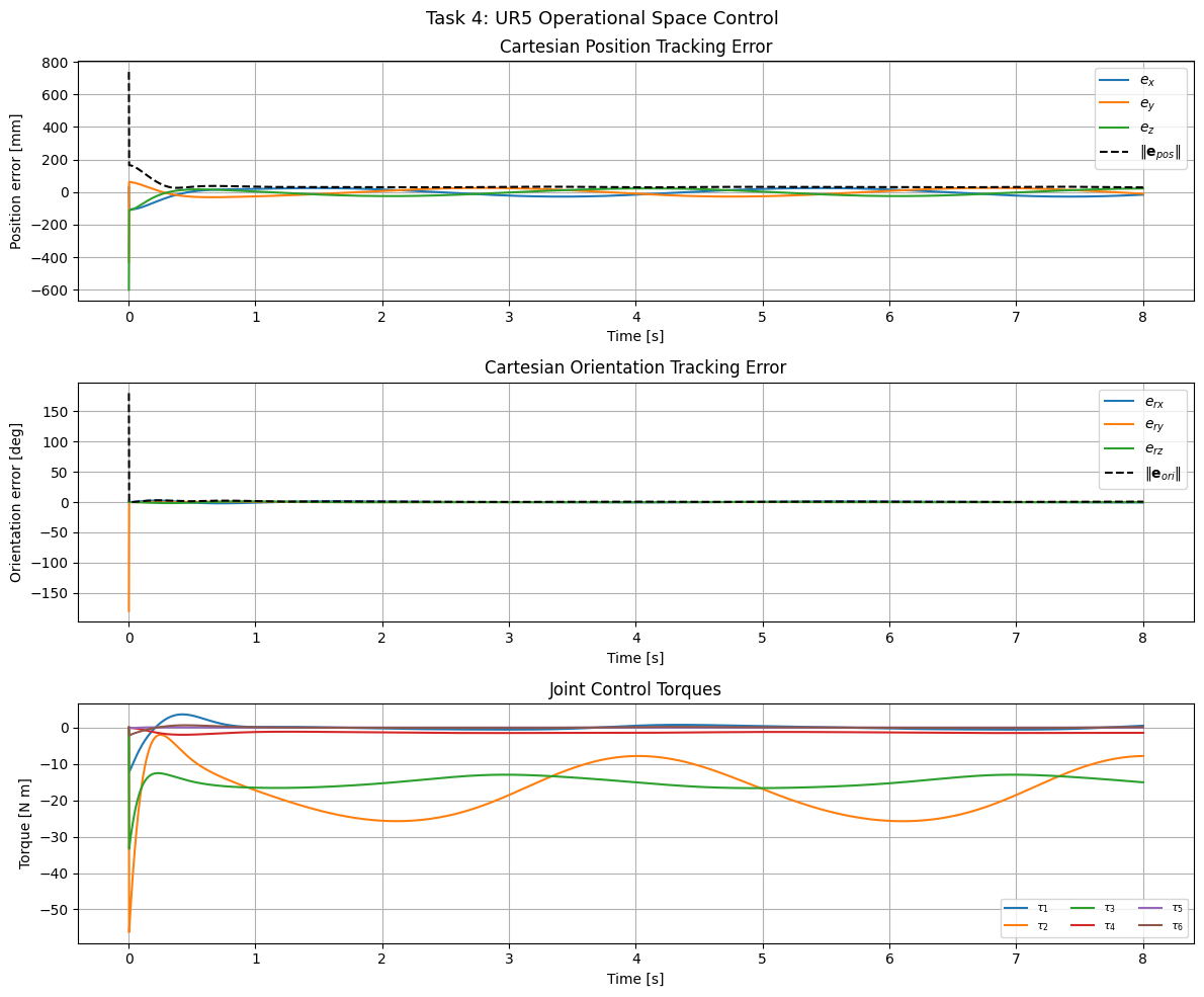
RMS position error:    39.11 mm
RMS orientation error: 2.996 deg
Problems
We will control the 3R spatial robot shown below. The robot has three revolute joints.
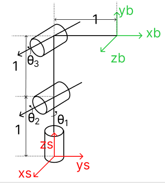
Each link has length m. The workspace is a 3D region (roughly a hemisphere of radius 3 m).
We first create and load the MuJoCo model, then implement two tasks:
Problem 1: Reach a random target point using PD control and Computed Torque Control
Problem 2: Track a 3D circular trajectory using Computed Torque Control (position only)
# -----------------------------------------------------------------------
# 3R Spatial Robot: MuJoCo XML and model loading
# -----------------------------------------------------------------------
# Robot structure (all links length = 1 m, mass = 1 kg):
#   Joint 1: pan  (Z-axis)  at base
#   Joint 2: pitch (Y-axis) at top of link 1
#   Joint 3: pitch (Y-axis) at top of link 2
#   End-effector: tip of link 3 (horizontal)

import mujoco, numpy as np, matplotlib.pyplot as plt, matplotlib
from IPython.display import HTML, display
matplotlib.use('Agg')

l1, l2, l3 = 1.0, 1.0, 1.0
m1, m2, m3 = 1.0, 1.0, 0.5

xml_3r = f"""
<mujoco model='3r_spatial'>
  <option gravity='0 0 -9.81' timestep='0.002' integrator='RK4'/>
  <compiler balanceinertia='true'/>
  <default>
    <joint damping='0' frictionloss='0'/>
    <motor ctrllimited='false'/>
  </default>

  <worldbody>
    <!-- Link 1: rotates about Z (pan), extends upward -->
    <body name='link1' pos='0 0 0'>
      <joint name='joint1' type='hinge' axis='0 0 1'/>
      <inertial pos='0 0 {l1/2}' mass='{m1}'
                diaginertia='{m1*l1**2/12:.4f} {m1*l1**2/12:.4f} 0.001'/>
      <geom type='capsule' fromto='0 0 0  0 0 {l1}' size='0.05' rgba='0.2 0.6 0.9 1' mass='0'/>

      <!-- Link 2: rotates about Y (pitch), extends upward -->
      <body name='link2' pos='0 0 {l1}'>
        <joint name='joint2' type='hinge' axis='0 1 0'/>
        <inertial pos='0 0 {l2/2}' mass='{m2}'
                  diaginertia='{m2*l2**2/12:.4f} {m2*l2**2/12:.4f} 0.001'/>
        <geom type='capsule' fromto='0 0 0  0 0 {l2}' size='0.04' rgba='0.9 0.5 0.2 1' mass='0'/>

        <!-- Link 3: rotates about Y (pitch), extends horizontally -->
        <body name='link3' pos='0 0 {l2}'>
          <joint name='joint3' type='hinge' axis='0 1 0'/>
          <inertial pos='{l3/2} 0 0' mass='{m3}'
                    diaginertia='0.001 {m3*l3**2/12:.4f} {m3*l3**2/12:.4f}'/>
          <geom type='capsule' fromto='0 0 0  {l3} 0 0' size='0.03' rgba='0.3 0.8 0.3 1' mass='0'/>
          <site name='end_effector' pos='{l3} 0 0' size='0.04' rgba='1 0 0 1'/>
        </body>
      </body>
    </body>
  </worldbody>

  <actuator>
    <motor name='tau1' joint='joint1'/>
    <motor name='tau2' joint='joint2'/>
    <motor name='tau3' joint='joint3'/>
  </actuator>
</mujoco>"""

with open('3r_spatial.xml', 'w') as f:
    f.write(xml_3r)

model   = mujoco.MjModel.from_xml_path('3r_spatial.xml')
data    = mujoco.MjData(model)
site_id = model.site('end_effector').id
print(f'Model loaded: {model.nv} DOF, timestep={model.opt.timestep} s')

# ---- Shared helper functions (reused in both problems) ----------------

def get_mass_matrix(model, data):
    """Joint-space inertia matrix M(q), shape (3,3)."""
    M = np.zeros((model.nv, model.nv))
    mujoco.mj_fullM(model, M, data.qM)
    return M

def get_ee_pos(data, site_id):
    """End-effector 3D position via MuJoCo forward kinematics."""
    return data.site(site_id).xpos.copy()

def get_jacobian(model, data, site_id):
    """Translational Jacobian J(q), shape (3,3): maps qdot -> ee velocity."""
    J_pos = np.zeros((3, model.nv))
    J_rot = np.zeros((3, model.nv))
    mujoco.mj_jacSite(model, data, J_pos, J_rot, site_id)
    return J_pos   # shape (3,3) for 3-DOF robot
Problem 1: Reaching Task
Goal: Drive the end-effector to a random reachable target position from an arbitrary initial configuration.
Steps:
Sample a random target inside the reachable workspace
Compute the desired joint angles (use MuJoCo or fix and solve analytically for )
Implement a joint-space PD controller:
Implement a joint-space computed torque controller:
Run both simulations from the same initial condition and compare
Hint: For gain design, use the same approach as Task 3.1: choose and , then , .
# -----------------------------------------------------------------------
# Problem 1: Reaching Task -- scaffold code
# -----------------------------------------------------------------------

# ---- TODO: Implement the PD controller --------------------------------
def pd_torque(data, q_d, Kp, Kd):
    """
    Joint-space PD controller (set-point, qdot_d = 0).
      tau = Kp*(q_d - q) + Kd*(0 - qdot)
    """
    # TODO: implement
    pass

# ---- TODO: Implement the Computed Torque controller ------------------
def ct_joint_torque(model, data, q_d, Kp, Kd):
    """
    Joint-space computed torque controller (set-point).
      tau = M(q)*(Kp*(q_d - q) + Kd*(0 - qdot)) + h(q, qdot)
    Hint: use get_mass_matrix() and data.qfrc_bias
    """
    # TODO: implement
    pass

# ---- Controller gains -------------------------------------------------
wn, zeta = 10.0, 0.9
Kp_ct = wn**2           # for CT
Kd_ct = 2*zeta*wn
Kp_pd = 400             # for PD: higher gains needed (no inertia cancellation)
Kd_pd = 50

# ---- Random reachable target ------------------------------------------
rng   = np.random.default_rng(seed=0)
# Workspace: sphere of radius (l1+l2+l3), avoid singularity near origin
r_tgt = rng.uniform(0.5, l1+l2+l3 - 0.1)
az    = rng.uniform(0, 2*np.pi)        # azimuth (joint 1 direction)
el    = rng.uniform(0, np.pi/2)        # elevation (above ground)
target_pos = r_tgt * np.array([np.sin(el)*np.cos(az),
                               np.sin(el)*np.sin(az),
                               np.cos(el)])
print(f'Target: {target_pos}')

# ---- TODO: Compute desired joint angles q_d via inverse kinematics ----
# Hint: fix q1 = arctan2(target_pos[1], target_pos[0]) for the pan angle,
# then the problem reduces to a 2R planar IK in the vertical plane.
# q1 = ?
# q2 = ?  (use 2R IK with the planar distance and height)
# q3 = ?
q_des = np.zeros(3)   # TODO: replace with IK solution

# ---- Simulation -------------------------------------------------------
q0    = np.array([0.0, np.pi/6, -np.pi/4])   # initial configuration
T_sim = 5.0
dt    = model.opt.timestep
n_steps = int(T_sim / dt)

def run_sim_p1(ctrl_fn):
    mujoco.mj_resetData(model, data)
    data.qpos[:] = q0;  data.qvel[:] = 0
    mujoco.mj_forward(model, data)
    t_l  = np.zeros(n_steps)
    q_l  = np.zeros((n_steps, 3))
    ee_l = np.zeros((n_steps, 3))
    tau_l = np.zeros((n_steps, 3))
    for k in range(n_steps):
        tau = ctrl_fn()
        data.ctrl[:] = tau
        mujoco.mj_step(model, data)
        t_l[k] = data.time
        q_l[k] = data.qpos.copy()
        ee_l[k] = get_ee_pos(data, site_id)
        tau_l[k] = tau
    return t_l, q_l, ee_l, tau_l

t_pd,  q_pd,  ee_pd,  tau_pd  = run_sim_p1(lambda: pd_torque(data, q_des, Kp_pd, Kd_pd))
t_ct,  q_ct,  ee_ct,  tau_ct  = run_sim_p1(lambda: ct_joint_torque(model, data, q_des, Kp_ct, Kd_ct))

# ---- Plot results (fill in) ------------------------------------------
fig, axes = plt.subplots(1, 3, figsize=(15, 4))
fig.suptitle('Problem 1: Reaching Task - PD vs CT', fontsize=12)

# TODO: plot joint angle errors, EE distance to target, control torques
# Hint: np.linalg.norm(ee_pd - target_pos, axis=1) gives EE distance over time

plt.tight_layout()
display(fig); plt.close(fig)
Problem 2: Trajectory Tracking (Position Only)
Goal: Track a 3D circular trajectory using computed torque control in operational space (position only, no orientation control).
Since the 3R robot has 3 joints and the task is 3D position (3 DOF), the translational Jacobian is square and invertible (away from singularities). The operational-space CT law is:
where is the 3D Cartesian position error.
Steps:
Define a 3D circle using the
circle_3dfunction (choose center, radius, normal vector)Implement the operational-space CT controller
Compare with the IK + joint-space CT approach (Method B from Task 3.2): compute , , from the trajectory at each step, then apply joint-space CT
Hint: Use np.linalg.solve(J, v) instead of np.linalg.inv(J) @ v for numerical stability. The term can be approximated numerically or dropped as a simplification.
# -----------------------------------------------------------------------
# Problem 2: Trajectory Tracking -- scaffold code
# -----------------------------------------------------------------------

# ---- 3D circle trajectory --------------------------------------------
def circle_3d(t, center, radius, normal, f):
    """3D circular trajectory: position, velocity, acceleration."""
    normal = normal / np.linalg.norm(normal)
    ref = np.array([0,0,1]) if abs(normal[2]) < 0.9 else np.array([1,0,0])
    u = np.cross(normal, ref);  u /= np.linalg.norm(u)
    v = np.cross(normal, u)
    w   = 2 * np.pi * f
    x_d   = center + radius * (np.cos(w*t)*u + np.sin(w*t)*v)
    xd_d  = radius * w  * (-np.sin(w*t)*u + np.cos(w*t)*v)
    xdd_d = radius * w**2 * (-np.cos(w*t)*u - np.sin(w*t)*v)
    return x_d, xd_d, xdd_d

# Trajectory parameters -- choose center inside the reachable workspace
traj_center = np.array([1.0, 0.0, 1.5])   # adjust as needed
traj_radius = 0.3
traj_normal = np.array([0, 0, 1])          # horizontal circle; try [1,0,0] or [1,1,0]
traj_f      = 0.2                           # Hz

# ---- TODO: Implement Method A -- Operational-Space CT ----------------
def ct_op_torque(model, data, x_d, xd_d, xdd_d, Kp, Kd):
    """
    Operational-space CT (position only):
      tau = M(q) J^{-1}(xdd_d + Kd*(xd_d - J*qdot) + Kp*(x_d - x) - Jdot*qdot) + h
    Note: Jdot*qdot can be set to zero as a simplification.
    Hint: use get_mass_matrix(), get_jacobian(), get_ee_pos(), data.qfrc_bias,
          and np.linalg.solve(J, v) to avoid explicit matrix inversion.
    """
    # TODO: implement
    pass

# ---- TODO: Implement Method B -- IK + Joint-Space CT -----------------
def ct_ik_joint_torque(model, data, x_d, xd_d, xdd_d, Kp, Kd):
    """
    IK + Joint-Space CT:
      Step 1: q_d   = IK(x_d)                        (desired joint angles)
              qd_d  = J^{-1} * xd_d                  (desired joint velocities)
              qdd_d = J^{-1} * (xdd_d - Jdot*qdot)   (desired joint accelerations)
      Step 2: tau = M(q)*(qdd_d + Kd*(qd_d-qdot) + Kp*(q_d-q)) + h
    Hint: for IK, fix q1 from the target azimuth angle, then apply 2R IK
          in the vertical plane for q2 and q3.
    """
    # TODO: implement
    pass

# ---- Controller gains (same for both methods) -------------------------
wn_t, zeta_t = 8.0, 1.0
Kp_t = wn_t**2
Kd_t = 2 * zeta_t * wn_t

# ---- Compute initial joint angles (start on the circle) --------------
x0, _, _ = circle_3d(0.0, traj_center, traj_radius, traj_normal, traj_f)
# TODO: compute q0_traj = IK(x0) so the robot starts on the trajectory
q0_traj = np.array([0.0, 0.5, -0.3])   # placeholder -- replace with IK

# ---- Simulation -------------------------------------------------------
T_traj  = 1.0 / traj_f * 2   # two full circles
n_steps = int(T_traj / model.opt.timestep)

def run_sim_p2(ctrl_fn):
    mujoco.mj_resetData(model, data)
    data.qpos[:] = q0_traj;  data.qvel[:] = 0
    mujoco.mj_forward(model, data)
    t_l   = np.zeros(n_steps)
    ee_l  = np.zeros((n_steps, 3))
    xd_l  = np.zeros((n_steps, 3))
    xe_l  = np.zeros((n_steps, 3))
    tau_l = np.zeros((n_steps, 3))
    for k in range(n_steps):
        x_d, xd_d, xdd_d = circle_3d(data.time, traj_center, traj_radius,
                                      traj_normal, traj_f)
        tau = ctrl_fn(x_d, xd_d, xdd_d)
        data.ctrl[:] = tau
        mujoco.mj_step(model, data)
        t_l[k]   = data.time
        ee_l[k]  = get_ee_pos(data, site_id)
        xd_l[k]  = x_d
        xe_l[k]  = x_d - get_ee_pos(data, site_id)
        tau_l[k] = tau
    return t_l, ee_l, xd_l, xe_l, tau_l

t_os,  ee_os,  xd_os,  xe_os,  tau_os  = run_sim_p2(
    lambda x_d, xd_d, xdd_d: ct_op_torque(model, data, x_d, xd_d, xdd_d, Kp_t, Kd_t))
t_ik,  ee_ik,  xd_ik,  xe_ik,  tau_ik  = run_sim_p2(
    lambda x_d, xd_d, xdd_d: ct_ik_joint_torque(model, data, x_d, xd_d, xdd_d, Kp_t, Kd_t))

# ---- Plot results (fill in) ------------------------------------------
fig, axes = plt.subplots(1, 3, figsize=(15, 5))
fig.suptitle('Problem 2: Trajectory Tracking - OS-CT vs IK+JS-CT', fontsize=12)

# TODO: plot (1) EE path vs desired circle (3D or XY projection)
#            (2) Cartesian tracking error norm over time
#            (3) Control torques
# Hint: np.linalg.norm(xe_os, axis=1)*1000 gives error magnitude in mm

plt.tight_layout()
display(fig); plt.close(fig)

rms_os = np.sqrt(np.mean(np.sum(xe_os**2, axis=1))) * 1000
rms_ik = np.sqrt(np.mean(np.sum(xe_ik**2, axis=1))) * 1000
print(f'RMS error -- OS-CT:    {rms_os:.2f} mm')
print(f'RMS error -- IK+JS-CT: {rms_ik:.2f} mm')