Lab9: RL: Value Iteration & Policy Iteration

# Minimal prerequisites
import numpy as np
import matplotlib.pyplot as plt

# Matplotlib: one chart per cell; no specific styles or colors set per instructions.
print("NumPy:", np.__version__)
print("Matplotlib:", plt.matplotlib.__version__)

# Define actions and their visual representations
ACTIONS = [0, 1, 2, 3, 4]  # up, right, down, left, stay
ACTION_ARROWS = {0:"↑", 1:"→", 2:"↓", 3:"←", 4:"*"} # For rendering the policy

class GridWorld:
    """
    A class to represent the Grid World environment.
    Manages the grid, states, actions, transitions, and rewards.
    """
    def __init__(self,
                 grid_shape=(5, 5),  # number of rows and columns
                 forbidden=None,
                 goal=None,
                 goal_reward=10.0,
                 step_reward=0.0,
                 forbidden_reward=-1.0,
                 boundary_reward=-1.0,
                 gamma=0.9):
        """
        Initializes the GridWorld environment.

        Args:
            grid_shape (tuple): The (rows, columns) of the grid.
            forbidden (list): A list of (row, col) tuples for forbidden states.
            goal (tuple): The (row, col) of the goal state.
            goal_reward (float): Reward for reaching the goal.
            step_reward (float): Reward for a standard step.
            forbidden_reward (float): Penalty for entering a forbidden state.
            boundary_reward (float): Penalty for hitting a wall or boundary.
            gamma (float): The discount factor for future rewards.
        """
        self.grid_shape = grid_shape
        # Default locations for forbidden cells and the goal if not provided
        self.forbidden = forbidden if forbidden is not None else [(1,1), (1,2),(2,2), (3,1), (3,3) ,(4,1)] # Example forbidden positions
        self.goal = goal if goal is not None else (3,2) # Example goal position

        # Reward structure
        self.goal_reward = goal_reward
        self.step_reward = step_reward
        self.forbidden_reward = forbidden_reward
        self.boundary_reward = boundary_reward

        # Discount factor
        self.gamma = gamma

    def in_bounds(self, s):
        """Check if a state 's' is within the grid boundaries."""
        r, c = s # r is the row, c is the column
        R, C = self.grid_shape # Total rows and columns
        return 0 <= r < R and 0 <= c < C # if within bounds then return True

    def is_forbidden(self, s):
        """Check if a state 's' is a forbidden cell."""
        return s in self.forbidden # if s is in forbidden list then return True

    def states(self):
        """Returns a list of all states in the grid."""
        R, C = self.grid_shape
        return [(r, c) for r in range(R) for c in range(C)]

    def step(self, s, a):
        """
        Performs a state transition based on the current state and action.
        This function defines the environment's dynamics.

        Args:
            s (tuple): The current state (row, col).
            a (int): The action to take.

        Returns:
            tuple: A tuple containing the next state (next_s) and the reward.
        """
        assert a in ACTIONS, f"Invalid action: {a}. Valid actions are: {ACTIONS}"

        r, c = s
        # Determine the next potential position based on the action
        if a == 0:    nr, nc = r-1, c    # up
        elif a == 1:  nr, nc = r, c+1    # right
        elif a == 2:  nr, nc = r+1, c    # down
        elif a == 3:  nr, nc = r, c-1    # left
        else:         nr, nc = r, c      # stay

        # Check for boundary collisions or walls
        if (not self.in_bounds((nr, nc))):
            next_s = s  # Agent stays in the same state
            reward = self.boundary_reward
        else:
            # The move is valid, so the agent moves to the new position
            next_s = (nr, nc)
            # Determine the reward based on the new state
            if next_s == self.goal:
                reward = self.goal_reward
            elif self.is_forbidden(next_s):
                reward = self.forbidden_reward
            else:
                reward = self.step_reward

        return next_s, reward

ACTION_ARROWS = {
    0: "↑",   # down
    1: "→",   # right
    2: "↓",   # up
    3: "←",   # left
    4: "•",   # stay
}

def render_policy_with_values(env, P, V=None, title="Policy and Values", ax=None, show=True):
    """
    Renders the greedy policy as arrows and overlays the value for each state in a matplotlib plot.

    Args:
        env: GridWorld environment object. Should provide .grid_shape and .is_forbidden().
        P (dict): The policy mapping states (r, c) to actions (int).
        V (dict): Optional. A dictionary mapping states to their values.
        title (str): Title of the plot.
        ax: Optional matplotlib axes object. If provided, plots on this axes instead of creating a new figure.
        show (bool): Whether to call plt.show() at the end. Default True. Set False when creating subplots.

    Returns:
        tuple: (fig, ax) - The figure and axes objects.
    """
    import matplotlib.pyplot as plt
    import numpy as np

    R, C = env.grid_shape
    if ax is None:
        fig, ax = plt.subplots(figsize=(7, 6))
    else:
        fig = ax.figure
    ax.set_xlim(-0.5, C - 0.5)
    ax.set_ylim(-0.5, R - 0.5)
    ax.set_xticks(np.arange(-0.5, C, 1))
    ax.set_yticks(np.arange(-0.5, R, 1))
    ax.grid(True, color='gray', linewidth=1, linestyle='-')
    ax.set_aspect('equal')
    ax.invert_yaxis()  # Match array indexing

    # Draw cell highlights for forbidden/goal/start
    for r in range(R):
        for c in range(C):
            s = (r, c)
            if env.is_forbidden(s):
                rect = plt.Rectangle((c-0.5, r-0.5), 1, 1, color='gray', alpha=0.5)
                ax.add_patch(rect)
                ax.text(c, r, "X", ha='center', va='center', color='black', fontsize=14)
            elif s == env.goal:
                rect = plt.Rectangle((c-0.5, r-0.5), 1, 1, color='yellow', alpha=0.45)
                ax.add_patch(rect)
                ax.text(c, r, "G", ha='center', va='center', color='black', fontsize=14)
            elif s == getattr(env, "start_state", None):
                rect = plt.Rectangle((c-0.5, r-0.5), 1, 1, color='deepskyblue', alpha=0.35)
                ax.add_patch(rect)
                ax.text(c, r, "S", ha='center', va='center', color='black', fontsize=14)

    # Print arrows and values in every cell (except forbidden)
    for r in range(R):
        for c in range(C):
            s = (r, c)
            # Print policy arrow
            if (r, c) in P:
                arrow = ACTION_ARROWS[P[(r, c)]]
            else:
                arrow = ""
            if (V is not None) and ((r, c) in V):
                valstr = f"{V[(r, c)]:.2f}"
            else:
                valstr = ""
            # Place arrow in cell
            ax.text(
                c, r-0.18, arrow,
                ha='center', va='center', color='darkblue', fontsize=22, fontweight='bold', zorder=10
            )
            # Always show value in each cell (if provided), not just if valstr != ""
            ax.text(
                c, r+0.27, valstr if valstr != "" else "",
                ha='center', va='center', color='crimson', fontsize=11, alpha=0.99,
                bbox=dict(facecolor="white", alpha=0.63, edgecolor='none', boxstyle='round,pad=0.16'),
                zorder=10
            )

    # Label grid
    for x in range(C):
        ax.text(x, -0.75, str(x+1), ha='center', va='center', color='black')
    for y in range(R):
        ax.text(-0.75, y, str(y+1), ha='center', va='center', color='black')

    ax.set_title(title)
    ax.tick_params(bottom=False, left=False, right=False, top=False,
                   labelbottom=False, labelleft=False, labeltop=False, labelright=False)
    if show:
        plt.tight_layout()
        plt.show()

    return fig, ax

def value_iteration(env, theta, max_iters):
    """
    Performs Value Iteration to find the optimal value function and policy,
    following the structure of the provided pseudocode.

    Args:
        env: The GridWorld environment.
        theta (float): A small threshold for determining convergence.
        max_iters (int): The maximum number of iterations to prevent infinite loops.

    Returns:
        tuple: A tuple containing:
            - V (dict): The optimal value function, mapping states to values.
            - Pi (dict): The optimal policy, mapping states to actions.
            - iters (int): The number of iterations until convergence.
    """
    # Initialization: Initial guess v0
    V = {s: 0.0 for s in env.states()}
    Pi = {s: 0 for s in env.states()} # Policy can be initialized arbitrarily
    iters = 0

    while True:
        delta = 0.0
        V_old = V.copy() # Store vk to calculate delta = ||vk - vk-1||

        # For every state s ∈ S, do
        for s in env.states():
            # For every action a ∈ A(s), do
            # q-value: qk(s, a) = r(s,a) + γ * V(s')
            q_values = {}
            for a in ACTIONS:
                s_next, r = env.step(s, a) # Get next state and reward
                q_values[a] = r + env.gamma * V_old[s_next] # get the action value

            # Maximum action value: a*k(s) = arg maxa qk(a, s)
            best_action = max(q_values, key=q_values.get)

            # Value update: vk+1(s) = maxa qk(a, s)
            best_value = q_values[best_action]
            V[s] = best_value

            # Policy update: πk+1(s) = a*k(s)
            Pi[s] = best_action

            # Check for convergence
            delta = max(delta, abs(V[s] - V_old[s]))

        iters += 1
        if delta < theta or iters >= max_iters:
            break

        # Show intermediate policy and values during value iteration
        # if iters % 20 == 0 or delta < theta:  # Visualize every 10 steps and at convergence
        #     render_policy_with_values(env, Pi, V, title=f"Value Iteration Step {iters}")
        #     import time
        #     time.sleep(1)
        #     plt.close('all')  # Close all existing figures before drawing a new one
    return V, Pi, iters

# Demo run
env = GridWorld()
V_vi, Pi_vi, n_vi = value_iteration(env, 1e-3, 1000)
print(f"Value Iteration converged in {n_vi} iterations.")
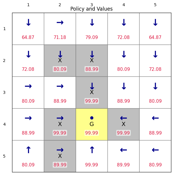
render_policy_with_values(env, Pi_vi, V_vi, title="Policy and Values")

def policy_evaluation(env, Pi, theta, max_iters):
    """
    Calculates the state-value function V for a given policy Pi.
    This is an iterative process that applies the Bellman equation until V converges.

    Args:
        env (GridWorld): The environment.
        Pi (dict): The policy to evaluate, mapping states to actions.
        theta (float): Convergence threshold. The loop stops when the max change in V is less than this.
        max_iters (int): Maximum number of iterations to prevent infinite loops.

    Returns:
        tuple: A tuple containing:
            - V (dict): The converged state-value function for the policy Pi.
            - iters (int): The number of iterations it took to converge.
    """
    # Initialize the value function V(s) = 0 for all states s.
    V = {s: 0.0 for s in env.states()}

    iters = 0
    while True:
        delta = 0.0  # Tracks the maximum change in V in a single sweep.
        V_old = V.copy() # Store the old value function for comparison.

        # Loop through each state to update its value.
        for s in env.states():
            # Get the action prescribed by the current policy for state s.
            a = Pi[s]

            # Get the next state and reward for the (s, a) pair.
            s_next, r = env.step(s, a)

            # Apply the Bellman equation for the given policy:
            # V(s) = R(s, a) + gamma * V(s_next)
            # This calculates the expected return from state s by following policy Pi.
            val = r + env.gamma * V_old[s_next]

            # Update the value for the current state.
            V[s] = val

            # Check for convergence by tracking the largest change in V.
            delta = max(delta, abs(val - V_old[s]))

        iters += 1
        # If the value function has stabilized, or we've hit the max iterations, stop.
        if delta < theta or iters >= max_iters:
            break

    return V, iters

def policy_improvement(env, V):
    """
    Improves a policy by making it greedy with respect to a given value function V.

    Args:
        env (GridWorld): The environment.
        V (dict): The value function to be greedy upon.

    Returns:
        dict: The new, improved policy.
    """
    Pi_new = {} # Initialize the new policy.

    # Iterate over all states to find the best action for each.
    for s in env.states():
        q_values = {}
        # For each state, calculate the Q-value for all possible actions.
        for a in ACTIONS:
            s_next, r = env.step(s, a)
            # Q(s, a) = R(s, a) + gamma * V(s_next)
            q_values[a] = r + env.gamma * V[s_next]

        # The new policy for state s will be the action that maximizes the Q-value.
        best_a = max(q_values, key=q_values.get)
        Pi_new[s] = best_a

    return Pi_new

def policy_iteration(env, theta, max_iters):
    """
    Performs Policy Iteration to find the optimal policy and value function.
    It alternates between Policy Evaluation and Policy Improvement until the policy converges.

    Args:
        env (GridWorld): The environment.
        theta (float): Convergence threshold for policy evaluation.
        max_iters (int): Maximum number of policy improvement steps.

    Returns:
        tuple: A tuple containing:
            - V (dict): The optimal value function.
            - Pi (dict): The optimal policy.
            - iteration (int): The number of policy improvement steps.
    """

    # Start with a random initial policy.
    # For each state, choose a random action from the set of possible actions.
    Pi = {s: np.random.choice(ACTIONS) for s in env.states()}
    iteration = 0

    while True:
        # Step 1: Policy Evaluation
        V, _ = policy_evaluation(env, Pi, theta, max_iters)

        # Step 2: Policy Improvement
        Pi_new = policy_improvement(env, V)
        iteration += 1

        # Step 3: Termination Check
        if Pi_new == Pi or iteration >= max_iters:
            break

        # Update the policy for the next iteration of the main loop.
        Pi = Pi_new

    # Return the final converged value function, policy, and number of iterations.
    return V, Pi_new, iteration

# --- Demo Run ---
# Create a new GridWorld instance for this demonstration.
env2 = GridWorld()

# Run the Policy Iteration algorithm.
V_pi, Pi_pi, iteration = policy_iteration(env2, theta=1e-5, max_iters=1000)

# Print the results and visualize the value function and policy.
print(f"Policy Iteration converged in {iteration} improvement steps.")
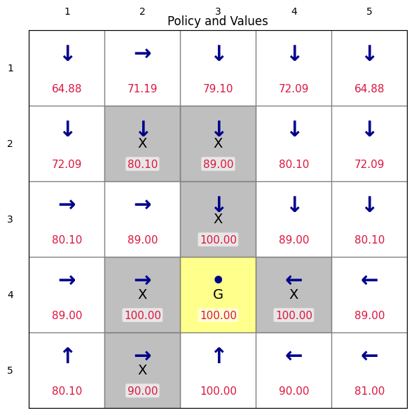
render_policy_with_values(env, Pi_pi, V_pi, title="Policy and Values")

# Quick side-by-side run for the same environment:
env_cmp = GridWorld(gamma=0.9)

V_vi, Pi_vi, n_vi = value_iteration(env_cmp, theta=1e-5, max_iters=1000)
V_pi, Pi_pi, n_pi = policy_iteration(env_cmp, theta=1e-5, max_iters=1000)

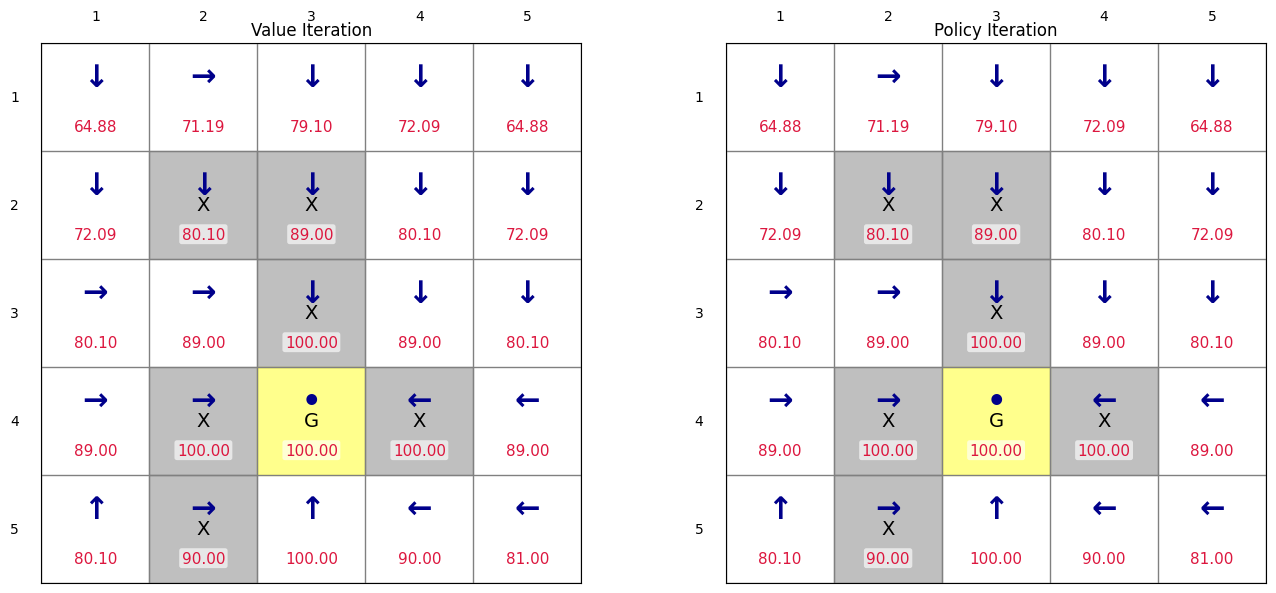
print(f"Value Iteration: {n_vi} iterations")
print(f"Policy Iteration: {n_pi} iterations")

import matplotlib.pyplot as plt

# Create a figure with two subplots side by side
fig, axes = plt.subplots(1, 2, figsize=(14, 6))

# Plot Policy from Value Iteration (left subplot)
render_policy_with_values(env_cmp, Pi_vi, V_vi, title="Value Iteration", ax=axes[0], show=False)

# Plot Policy from Policy Iteration (right subplot)
render_policy_with_values(env_cmp, Pi_pi, V_pi, title="Policy Iteration", ax=axes[1], show=False)

plt.tight_layout()
plt.show()

try:
    import gymnasium as gym
except ModuleNotFoundError:
    import sys
    !{sys.executable} -m pip install gymnasium
    import gymnasium as gym
from gymnasium import spaces # spaces are used to define action and observation spaces
import numpy as np

# Define the set of possible actions and their visual representations
ACTIONS = [0, 1, 2, 3, 4]  # up, right, down, left, stay
ACTION_ARROWS = {0:"↑", 1:"→", 2:"↓", 3:"←", 4:"*"}


class GridWorldEnv(gym.Env):
    """Custom GridWorld environment compatible with Gymnasium API."""
    """Note that Gymnasium environments are typically implemented as classes that inherit from gym.Env.
    This allows them to integrate seamlessly with the Gymnasium framework,
    which provides tools for reinforcement learning research and development."""
    """You may compare this class with the one implemented at the beginning as a simple GridWorld class.
    The only difference is that this class follows the Gymnasium API requirements: it defines action_space and observation_space,
    and implements reset() and step() methods."""

    def __init__(self,
                 grid_shape=(5, 5),
                 forbidden=None,
                 goal=None,
                 goal_reward=1.0,
                 step_reward=0.0,
                 forbidden_reward=-10.0,
                 boundary_reward=-1.0,
                 gamma=0.9,
                 render_mode=None):
        """
        Initializes the GridWorld environment.

        Args:
            grid_shape (tuple): The shape of the grid (rows, columns).
            forbidden (list of tuples): A list of coordinates for forbidden states.
            goal (tuple): The coordinates of the goal state.
            goal_reward (float): The reward for reaching the goal.
            step_reward (float): The reward for a regular step.
            forbidden_reward (float): The reward for entering a forbidden state.
            boundary_reward (float): The reward for hitting a boundary.
            gamma (float): The discount factor for future rewards.
            render_mode (str, optional): The mode for rendering the environment.
        """
        super().__init__()

        # Environment parameters
        self.grid_shape = grid_shape
        self.forbidden = forbidden if forbidden is not None else [(2,2)]
        self.goal = goal if goal is not None else (4,4)
        self.goal_reward = goal_reward
        self.step_reward = step_reward
        self.forbidden_reward = forbidden_reward
        self.boundary_reward = boundary_reward
        self.gamma = gamma
        self.render_mode = render_mode

        # Agent's current position, initialized in reset()
        self.agent_pos = None

        # Define Gymnasium spaces
        # The action space is discrete with a size equal to the number of actions.
        self.action_space = spaces.Discrete(len(ACTIONS))
        # The observation space represents the agent's position on the grid.
        self.observation_space = spaces.MultiDiscrete(list(grid_shape))

    # -----------------------------------
    # Helper functions
    # -----------------------------------
    def in_bounds(self, s):
        """Check if a state 's' is within the grid boundaries."""
        r, c = s
        R, C = self.grid_shape
        return 0 <= r < R and 0 <= c < C

    def is_forbidden(self, s):
        """Check if a state 's' is a forbidden state."""
        return s in self.forbidden

    def states(self):
        """Return a list of all possible states (coordinates) in the grid."""
        valid_states = []
        R, C = self.grid_shape
        for r in range(R):
            for c in range(C):
                valid_states.append((r,c))
        return valid_states

    # -----------------------------------
    # Gymnasium required methods
    # -----------------------------------

    def reset(self, seed=None, options=None):
        """
        Reset the environment to its initial state.
        The agent is placed at the starting position (0,0).
        Returns the initial observation and an info dictionary.
        """
        super().reset(seed=seed)
        self.agent_pos = (0, 0)   # Always start in the top-left corner
        # The observation is the agent's position as a numpy array.
        obs = np.array(self.agent_pos, dtype=np.int32)
        return obs, {}

    def step(self, action):
        """
        Execute one time step in the environment.
        The agent takes an action, and the environment transitions to a new state.

        Args:
            action (int): The action to be taken by the agent.

        Returns:
            tuple: A tuple containing the new observation, the reward,
                   a boolean indicating if the episode is terminated,
                   a boolean indicating if the episode is truncated,
                   and an info dictionary.
        """
        assert self.action_space.contains(action), f"Invalid action {action}"

        r, c = self.agent_pos

        # Map the action to a new position (nr, nc for new row, new col)
        if action == 0:    nr, nc = r - 1, c     # up
        elif action == 1:  nr, nc = r, c + 1     # right
        elif action == 2:  nr, nc = r + 1, c     # down
        elif action == 3:  nr, nc = r, c - 1     # left
        else:              nr, nc = r, c         # stay

        # Check for environment boundaries
        if not self.in_bounds((nr, nc)):
            next_pos = self.agent_pos  # Agent stays in the same position
            reward = self.boundary_reward
        else:
            # The new position is valid
            next_pos = (nr, nc)
            # Assign reward based on the new state
            if next_pos == self.goal:
                reward = self.goal_reward
            elif self.is_forbidden(next_pos):
                reward = self.forbidden_reward
            else:
                reward = self.step_reward

        # Update the agent's position
        self.agent_pos = next_pos

        # Prepare the return values
        obs = np.array(self.agent_pos, dtype=np.int32)

        # In this simple environment, an episode never terminates or gets truncated on its own.
        # This would be different in environments with terminal states or time limits.
        terminated, truncated, info = False, False, {}

        return obs, reward, terminated, truncated, info

def value_iteration_gym(env, theta, max_iters):
    """
    Performs Value Iteration for a Gymnasium-based GridWorld environment.
    This implementation is similar to the one in Task 2.

    Args:
        env (GridWorldEnv): The Gymnasium-style GridWorld environment.
        theta (float): A small threshold for determining convergence.
        max_iters (int): The maximum number of iterations.

    Returns:
        tuple: A tuple containing:
            - V (dict): The optimal value function.
            - Pi (dict): The optimal policy.
            - iters (int): The number of iterations until convergence.
    """
    # Initialization
    states = env.states()
    V = {s: 0.0 for s in states}
    Pi = {s: 0 for s in states}  # Arbitrary initial policy
    iters = 0

    while True:
        delta = 0.0
        V_old = V.copy()  # Store the value function from the previous iteration

        # Loop over all states
        for s in states:
            q_values = {}
            # Calculate the q-value for each action in the current state
            for a in ACTIONS:
                # The Gym env is stateful, so we need to set its position to the state 's' we are evaluating
                env.agent_pos = s
                # The step function returns the next state and reward
                s_next_arr, r, _, _, _ = env.step(a)
                s_next = tuple(s_next_arr) # Convert numpy array to tuple for dict key

                # Bellman update using the value function from the *previous* iteration
                q_values[a] = r + env.gamma * V_old[s_next]

            # Find the best action and its value
            best_action = max(q_values, key=q_values.get)
            best_value = q_values[best_action]

            # Update the value function and policy for the current state
            V[s] = best_value
            Pi[s] = best_action

            # Track the maximum change in the value function for convergence check
            delta = max(delta, abs(V[s] - V_old[s]))

        iters += 1
        # Check for convergence
        if delta < theta or iters >= max_iters:
            break

    return V, Pi, iters

# ---- Demo Run ----
env = GridWorldEnv()
V_vi, Pi_vi, n_vi = value_iteration_gym(env, theta=1e-3, max_iters=1000)
print(f"Value Iteration converged in {n_vi} iterations.")
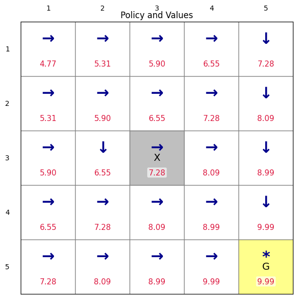
render_policy_with_values(env, Pi_vi, V_vi, title="Policy and Values")