In this chapter, we will talk about the actuators for robots. If you want to build a robot, the first question is to decide what kind of actuators that you will use. In most cases, this means what kind of motor you will use. Directly controlling a motor used to be relatively complicated. For instance, you can use a motor driver to control the direction and speed of a motor. Or you can simply use a stepper motor that does not have feedback, or a DC motor with a seperate encoder. You might also need to design a PID controller to control the motor’s position or velocity. Each of this is nontrival.
Recently, there are various integrated and low-cost smart actuators that we can directly use. Such smart actuators integrate everything you need in a compact package, including DC motor, encoder, control circuit, and also control algorithms implemented. This types of motor is initiated by a company called Robotis with their flagship motor series Dynamixel. Another popular one is from FeeTech due to the widely popular open source robotic arm SO-ARM 101 developed by HuggingFace.
Since the actuators already has everything it needed to control the motor, all you need to do is to send the command (desired angles or velocity) from a laptop (or single board computers like Raspberry Pi ) through a comunbication board to the controller inside these acuators. This significantly minimizes the effort to use motors for robotic applications.
In this book, we will discuss the following two types of actuators
Smart Bus servo motors
Quasi direct drive motors
These two types of actuators have enabled many open-source robot designs. A few recent and notable ones are as follows:
XLeRobot: two SO-ARM 101 on a movable IKEA cart, enabling mobile manipulation with a cost around $660.
Open Duck: a miniature version of the BDX Droid by Disney. It is about 42 centimeters tall with its legs extended. The cost is around $400.
OpenArm: a fully open-source humanoid robot arm designed for physical AI research and deployment in contact-rich environments.
reBot- DevArm: a robotic arm project dedicated to lowering the barrier to learning Embodied AI.
MicroDuck: A tiny biped robot you can teach new tricks.
2.1 DC Motors¶
Before looking at the integrated “smart” actuators, it’s worth understanding the motor that lives inside almost all of them: the DC motor. Bus servos, quasi-direct-drive actuators, and most stepper-driven systems are, underneath the electronics, a DC (or permanent-magnet synchronous) motor wrapped in a gearbox, an encoder, and a control loop. Understanding how a bare DC motor trades torque for speed — and what the numbers on a datasheet actually mean — makes it much easier to reason about any actuator you plug into a robot, smart or not.
2.1.1 Brushed and Brushless DC Motors¶
A DC motor produces torque the same way regardless of its construction: a current-carrying coil sits in a magnetic field, and the Lorentz force on the current turns that field into a torque on the rotor. The two common motor families differ only in how the current gets switched as the rotor turns — a step called commutation.
Brushed DC motors put the permanent magnets on the stationary housing (the stator) and the current-carrying windings on the rotating part (the rotor, or armature). A mechanical commutator — a set of copper contacts on the rotor — and spring-loaded brushes that ride against it switch the current direction in each winding as the rotor spins, so the torque always pushes the rotor the same way. Applying voltage to a brushed motor makes it spin; reversing the voltage reverses it. That simplicity is the whole appeal — a brushed motor needs nothing more than an H-bridge to drive. The following video explains the working principle of brushed DC motor.
Brushless DC motors (BLDC) flip the arrangement: the permanent magnets are on the rotor, and the windings stay on the stator. With nothing to commutate mechanically, an electronic motor driver (ESC) does the job instead — it senses rotor position (with Hall-effect sensors, or by measuring the back-EMF on the undriven phase) and energizes the stator windings in the right sequence to keep the torque pushing the right way. The following video explains the working principle of a BLDC.
| Brushed DC | Brushless DC (BLDC) | |
|---|---|---|
| Commutation | Mechanical (brushes + commutator) | Electronic (driver + rotor-position sensing) |
| Driver electronics | Simple — just an H-bridge | More complex — a 3-phase driver/ESC |
| Efficiency | Lower (brush friction, sparking losses) | Higher — no brush losses |
| Lifespan | Limited by brush wear | Long — no wearing contacts |
| Heat dissipation | Windings on the rotor, harder to cool | Windings on the stator, easier to cool |
| Cost | Cheap | More expensive (magnets + driver) |
| Typical robotics use | Small toy/hobby drivetrains, simple actuators | Quasi-direct-drive actuators, drones, high-performance drivetrains |
For most robotics work you rarely drive a bare DC motor at all — you buy it already paired with a gearbox and encoder as a gearmotor, or fully integrated with a driver and control loop as a smart actuator (Sections 2.2–2.3). But the torque–speed behavior described next is common to both families, and it’s what actually determines whether a given motor can do the job.
2.1.2 Key Parameters and the Torque–Speed Curve¶
A DC motor’s steady-state behavior is captured by two simple relationships. Electrically, the applied voltage splits between the resistive drop across the winding and the back-EMF generated by the spinning rotor:
Mechanically, the torque produced is proportional to current:
where is the torque constant and is the back-EMF constant — in SI units (N·m/A and V·s/rad) they are numerically equal, so many datasheets just report a single “motor constant” . is a small torque lost to bearing/brush friction; it’s what makes a motor draw current even when it’s spinning free.
Combining the two equations gives the motor’s torque–speed line at a fixed voltage :
When , i.e., the motor is stalled, we have the stall torque . When the torque is zero, we have the no-load speed . Note that motor companies will always provide the values for and . In this case, it is beneficial to rewrite the equation in terms of those two endpoints ( and ) instead of the four physical constants , , , :
This is the same line, just reparameterized. Every DC motor operates somewhere on this line — or, at a lower voltage, on a line parallel to and below it.
| Symbol | Meaning | Typical units |
|---|---|---|
| Rated terminal voltage | V | |
| Winding (terminal) resistance | Ω | |
| Torque constant | N·m/A | |
| Back-EMF constant ( in SI) | V·s/rad | |
| Stall current (current at ) | A | |
| Stall torque — max torque, at zero speed | N·m | |
| No-load current (friction losses) | A | |
| No-load speed — max speed, at zero torque | rad/s (or RPM) | |
| , | Continuous-duty torque/current the motor can sustain without overheating | N·m, A |
The single most common mistake when picking a motor is designing around stall torque instead of continuous (rated) torque. Stall torque is only available for a few seconds before the windings overheat — as a rule of thumb, continuous torque is often only 15–25% of stall torque. Size a motor for the torque it must hold up continuously; stall torque is your margin for brief accelerations, not your operating point.
The plot below lets you explore how , , , and the no-load current shape the torque, power, and efficiency curves. Two things worth noticing: peak mechanical power occurs at the midpoint of the torque–speed line (), while peak efficiency occurs at a higher speed, closer to — because efficiency is hurt by resistive () losses at high current/low speed just as much as it’s hurt by a vanishing torque near no load.
import numpy as np
import matplotlib.pyplot as plt
%matplotlib inline

def plot_dc_motor_curves(V=12.0, R=1.5, Kt=0.03, I0=0.05):
    """Torque, power, and efficiency vs. speed for a DC motor at fixed voltage V."""
    Ke = Kt  # SI units: torque and back-EMF constants are numerically equal
    omega_nl = (V - I0 * R) / Ke              # actual no-load speed (tau = 0)
    omega = np.linspace(0, omega_nl, 400)

    I = (V - Ke * omega) / R
    tau = Kt * (I - I0)
    tau = np.clip(tau, 0, None)
    P_out = tau * omega
    P_in = V * I
    eta = np.divide(P_out, P_in, out=np.zeros_like(P_out), where=P_in > 0) * 100

    tau_stall = tau[0]
    i_pmax = np.argmax(P_out)
    i_emax = np.argmax(eta)

    fig, axes = plt.subplots(1, 3, figsize=(14, 4))

    axes[0].plot(omega, tau, color='tab:blue')
    axes[0].axvline(omega[i_pmax], color='gray', ls='--', lw=1)
    axes[0].set_title(f'Torque vs. Speed\n$\\tau_{{stall}}$={tau_stall:.3f} N*m, $\\omega_{{nl}}$={omega_nl:.1f} rad/s')
    axes[0].set_xlabel('Speed $\\omega$ (rad/s)')
    axes[0].set_ylabel('Torque (N*m)')

    axes[1].plot(omega, P_out, color='tab:green')
    axes[1].axvline(omega[i_pmax], color='gray', ls='--', lw=1)
    axes[1].set_title(f'Output Power vs. Speed\nmax P={P_out[i_pmax]:.2f} W at $\\omega$={omega[i_pmax]:.1f} rad/s')
    axes[1].set_xlabel('Speed $\\omega$ (rad/s)')
    axes[1].set_ylabel('Power (W)')

    axes[2].plot(omega, eta, color='tab:red')
    axes[2].axvline(omega[i_emax], color='gray', ls='--', lw=1)
    axes[2].set_title(f'Efficiency vs. Speed\nmax $\\eta$={eta[i_emax]:.1f}% at $\\omega$={omega[i_emax]:.1f} rad/s')
    axes[2].set_xlabel('Speed $\\omega$ (rad/s)')
    axes[2].set_ylabel('Efficiency (%)')
    axes[2].set_ylim(0, 100)

    for ax in axes:
        ax.grid(alpha=0.3)
    plt.tight_layout()
    plt.show()

# Static snapshot at representative default values (V=12 V, R=1.5 Ohm, Kt=0.03 N*m/A, I0=0.05 A).
# The live notebook version of this cell lets you sweep V, R, Kt, and I0 with sliders;
# download the notebook (or open it in Binder/Colab) and run it locally to explore that interactively.
plot_dc_motor_curves()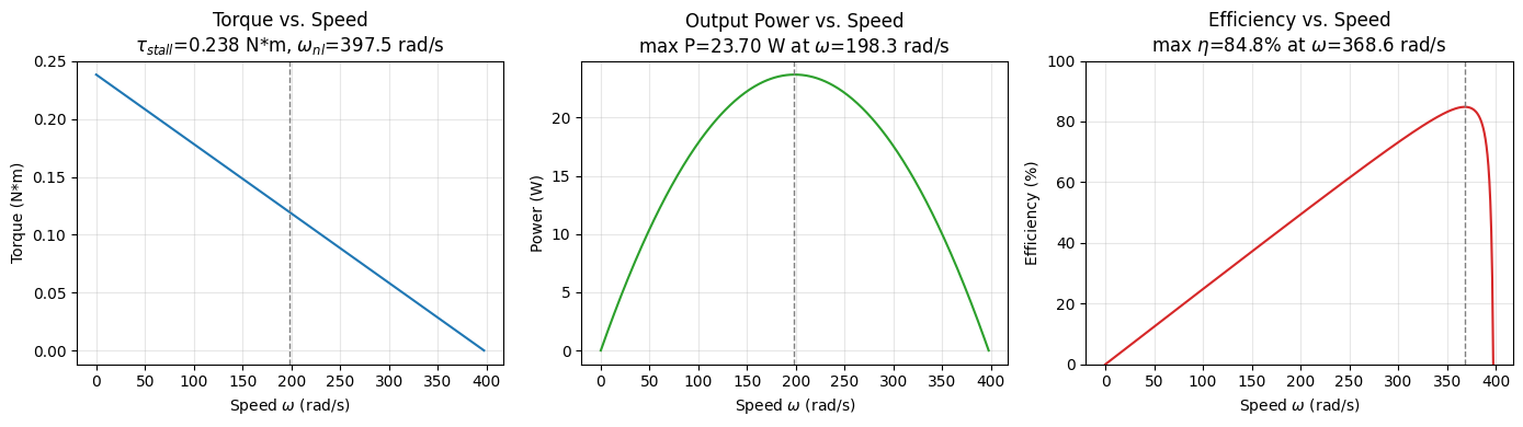
2.1.3 Choosing a Motor: Two Examples¶
Picking a motor is an exercise in working backward from what the joint or wheel needs to do, then checking that against a candidate motor’s torque–speed line — not just comparing a single “torque” number on a spec sheet.
Example 1 — A robot wrist/gripper joint, picked from a real motor family
Suppose a wrist/gripper joint needs to hold a link + payload with combined mass kg at a reach of m, worst case with the joint horizontal. The required holding torque at the joint is
and the joint should be able to sweep at up to — in RPM, that’s
Assume you are allowed to choose one motor from the following table, which one should you choose?
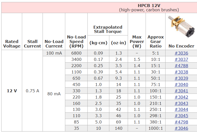
All thirteen rows share the same 12 V core motor; only the gear ratio differs, so No-Load Speed and Extrapolated Stall Torque are already output-shaft numbers — unlike a bare motor, there’s no separate step to add, since the gearbox is already built in. The datasheet doesn’t publish a continuous rating, so apply the same rule of thumb from §2.1.2 anyway: size against roughly 15–25% of stall, not stall itself.
Scanning down the table, the low gear ratios spin fast but can’t supply much torque, and torque only grows as the ratio climbs — so pick the smallest ratio whose derated stall still clears 0.025 N·m, rather than paying for more torque (and losing speed) than the joint needs. The 100:1 row ( kg·cm, RPM) is that motor:
kg·cm
which is just enough to meet the 0.25 kg·cm requirement. (One ratio down, 75:1, derates to only 0.20 kg·cm and falls short — so 100:1 really is the minimum viable choice here)
It’s still worth checking the actual operating point on the torque–speed line, rather than trusting the two extremes (stall and no-load) independently — Example 2 below shows a case where that check matters a lot. Recall from §2.1.2 that the torque–speed line is just the straight line connecting to :
Solving this for at a given torque just rearranges that line:
The datasheet already gives directly in RPM, so — unlike before — there’s no unit conversion to do first: the formula works the same regardless of which speed unit and share, as long as they match. Plugging in kg·cm, kg·cm, and RPM directly:
— far above the 15 RPM target. Notice the pattern across the whole family: torque is consistently the binding constraint, and speed comes along for free — even the smallest ratio strong enough to hold the load ends up wildly over-provisioned on speed.
Example 2 — A mobile robot drivetrain, a different row from the same table
A two-wheel-drive robot of mass kg with wheel radius m needs a top speed of m/s and should accelerate at on flat ground with rolling-resistance coefficient . Per wheel, the tractive force needed during acceleration is
so the required wheel torque is N·m, and the required wheel speed is .
This time pick a different row from the same table: the 210:1 gearmotor ( kg·cm N·m, RPM rad/s). As in Example 1, check the continuous rating first, not stall itself:
— comfortably above the 0.042 N·m required, about 17% of margin. But clearing the torque check doesn’t automatically mean the speed is there too — check where 0.042 N·m sits on the actual torque–speed line:
That’s just above the 13.3 rad/s needed — the motor is barely adequate on speed, even though it cleared the torque check with room to spare.
The neighboring rows fail for two different reasons. One ratio down, 150:1 ( N·m, rad/s): N·m, short of the 0.042 N·m required — this one fails the torque check before speed is ever in question, even though the raw torque–speed line would have given it speed to spare ( rad/s at 0.042 N·m). One ratio up, 250:1 ( N·m, rad/s): N·m clears the torque requirement by an even wider margin than 210:1 — but the operating point drops to only rad/s, so it fails on speed instead. Only 210:1 clears both checks, which is exactly why the continuous-torque check and the operating-point check are two separate, necessary steps: passing one doesn’t guarantee the other.
Key Takeaways — Section 2.1
Brushed motors commutate mechanically (brushes + commutator); brushless motors commutate electronically and are more efficient and longer-lived, at the cost of driver complexity.
A motor’s behavior at a given voltage is a straight torque–speed line from stall torque (at ) to no-load speed (at ); peak mechanical power is at the midpoint, peak efficiency is closer to no-load speed.
Size a motor by its continuous (rated) torque, not stall torque — stall torque is only a short-term margin.
When gearing/wheels are involved, check the required operating point against the actual torque–speed line, not stall torque and no-load speed independently — a motor can look overspec’d on one axis and be marginal on the other.
2.2 Smart Bus Servo Motors¶
If you want to directly use a DC motor from the ground up to precisely control the position and speed, you generally need a separate encoder to sense position, a driver to switch current, and controller to implement a PID loop to make it go to a desired angle or track a speed. A smart bus servo is exactly that stack — motor, gearbox, encoder, driver, and control loop — built into a single sealed unit that you talk to over a two-wire digital bus. You send it a target (an angle, a speed) and an address; it handles the rest, and reports back how it’s actually doing. This is the actuator family used throughout the labs in this book, including every joint of the SO-ARM101.
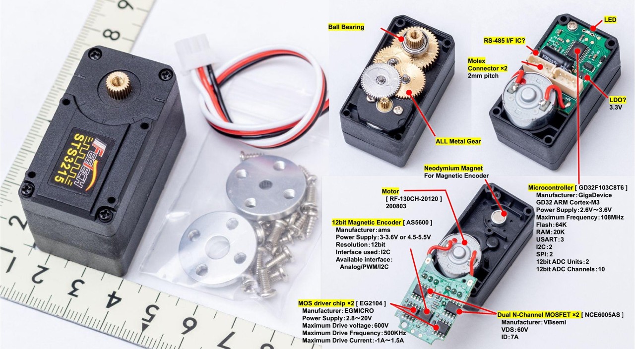
Figure 2.1: A FeeTech STS3215 smart bus servo (the motor used in the SO-ARM101) disassembled. Inside the case: an all-metal reduction gear stage, a 12-bit magnetic encoder, a small brushed DC motor, and a PCB with a microcontroller, driver MOSFETs, and an RS-485 interface — everything needed to close a position loop, packaged as one unit.
2.2.1 Anatomy of a Smart Bus Servo¶
Figure 2.1 shows a FeeTech STS3215 opened up — the four subsystems inside every smart bus servo:
A small brushed DC motor (labeled “Core Motor” on the datasheet) — everything from Section 2.1 applies to it directly.
A metal reduction gear train — copper gears riding on ball bearings, stepping the motor’s high speed / low torque down to a low speed / high torque suitable for a joint.
A 12-bit magnetic encoder mounted on the output shaft, not the motor shaft — it reads absolute output position directly, with resolution, and doesn’t lose track of position across the gear train the way an encoder on the motor shaft would.
A control PCB carrying a microcontroller, the driver MOSFETs that switch current to the motor, and a half-duplex serial transceiver for the communication bus.
All of that is packaged in a case about the size of a couple of AA batteries. Here are the numbers for the 12 V, 30 kg·cm variant (FeeTech ST-3215-C047) used as our running example:
| Parameter | Value |
|---|---|
| Rated voltage | 12 V (operable 4–14 V) |
| Stall torque | 30 kg·cm ≈ 2.94 N·m |
| Rated (continuous) torque | 10 kg·cm ≈ 0.98 N·m |
| No-load speed | 45 RPM ≈ 4.7 rad/s |
| Stall current | 2.7 A |
| Rated current | 0.9 A |
| Terminal resistance | 1.0 Ω |
| Torque constant | 11 kg·cm/A (at the output shaft, after the gearbox) |
| Gear ratio | 345:1 |
| Position resolution | 12-bit, 0.088°/count |
| Weight | 55 g |
Compare that stall torque — nearly 3 N·m — to the small hobby gearmotors in Section 2.1’s Example 1, which topped out around 10 kg·cm (≈1 N·m) only at their highest 1000:1 ratio. The STS3215’s 345:1 gearbox delivers three times that torque at a fraction of the ratio, thanks to a beefier core motor — at the cost of speed (45 RPM is slow) and reduced backdrivability.
2.2.2 Under the Hood: Closed-Loop Control and Protection¶
The datasheet lists the servo’s control algorithm simply as “PID, customizable.” In practice this is a cascade of loops — a position loop that outputs a velocity command, feeding an inner current loop that decides how much current to push into the motor — rather than one single PID acting directly on motor voltage. This loop runs entirely inside the servo, at an high update rate the host computer never has to keep up with.
That closed loop also explains something that looks odd if you apply Section 2.1’s equations directly. Using V and from the table above, the raw electrical stall current would be
but the datasheet’s actual stall current is only 2.7 A — the driver is actively current-limiting, not just relying on the winding’s resistance to hold current down. And it doesn’t hold even that current forever: if the servo is still stalled after 2 seconds, an overcurrent protection trips and shuts the output off entirely, on top of separate overvoltage (outside 4–14 V) and overtemperature (>70°C) cutouts. A bare DC motor from Section 2.1 has none of this — stall it and it will happily draw its full current until something overheats. “Smart” here means the actuator is actively protecting itself, not just executing commands.
2.2.3 Control Modes¶
A bus servo can be configured into different operating modes, changing what a command actually means:
| Mode | Name | Behavior |
|---|---|---|
| 0 | Position (servo) mode — default | Drive to an absolute angle, 0–, 4096 counts of resolution |
| 1 | Closed-loop velocity mode | Track a target speed; the internal loop compensates for load, so speed stays roughly constant as torque demand increases |
| 2 | Open-loop velocity mode | Apply a target duty cycle only; speed sags under load, following the raw torque–speed line from Section 2.1 |
| 3 | Step mode | Move a relative number of steps from the current position |
Modes 1 and 2 are a nice illustration of what feedback buys you: mode 2 is a bare motor’s torque–speed line — as load torque increases, speed drops linearly, exactly like the plot in Section 2.1.2. Mode 1 uses the encoder to detect that sag and increases current to fight it, holding speed nearly constant until the servo runs out of torque entirely. There’s also a multi-turn mode, extending position tracking to full revolutions (useful for continuously-geared joints), though the turn count isn’t retained across a power cycle.
2.2.4 Talking to a Servo: Protocol and Wiring¶
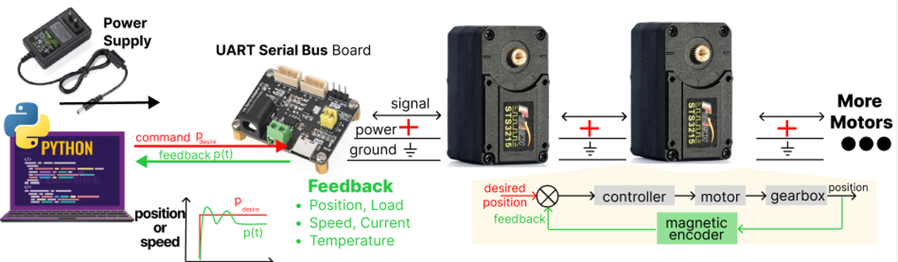
Communication happens over a half-duplex, packet-based serial protocol — a single wire carries both directions, one device transmitting at a time. Each servo is configured with a unique ID (0–253), and the host addresses individual servos on a shared bus rather than needing a dedicated wire per motor. Default baud rate is 1 Mbps (configurable down to 38.4 kbps), and a command packet can update a servo’s target roughly every 1 ms.
The minimal hardware setup is: a laptop (or microcontroller) connected through a USB-to-TTL/RS-485 adapter board, wired to the servo’s 3-pin connector — ground, power, and a single signal/data line. This is illustrated in the following fgiure.
2.2.5 Daisy-Chaining for Multi-DOF Systems¶
Because every servo on the bus has its own ID, many servos can share the same two signal wires and power rail — the host just addresses whichever one it wants to command. Chain the servos’ connectors together and a 6-joint arm needs one communication line and one power rail total, instead of six independent control connections. This is the main reason bus servos are so common in arms and legged robots: wiring complexity stops scaling with the number of joints.
The catch is power, not signal. Daisy-chaining passes both power and ground link-to-link, and each servo can briefly draw its full stall current — for six servos on our example part, that’s up to if they all load up at once (e.g., an arm catching a load, or several joints holding against gravity at once). Thin daisy-chain wiring and a single power injection point will show real voltage sag under that kind of transient draw, which can brown out the servos’ logic. The usual fix is to inject power at more than one point along the chain (thicker gauge wire, multiple taps back to the supply) rather than relying on the signal cable’s own conductors to carry it end-to-end.
Key Takeaways — Section 2.2
A smart bus servo packages a DC motor, gearbox, encoder, driver, and closed-loop controller into one unit — everything Section 2.1 required you to assemble by hand.
Its gearbox trades speed for torque (e.g., 345:1 turning a small motor into ~30 kg·cm at the output); its magnetic encoder reads output position directly, not motor position.
The internal control loop does more than track a setpoint — it also protects the actuator (current, voltage, and thermal limits), which is why real stall current is well below the naive prediction.
Position, velocity, and step modes change what a command means; closed-loop velocity mode is the feedback fix for the open-loop torque–speed droop from Section 2.1.
A shared, addressable serial bus lets many servos daisy-chain on one signal line — but power still needs enough headroom (and injection points) for several servos drawing current at once.
2.3 Quasi Direct Drive (QDD) Motors¶
Section 2.2’s bus servo is excellent at holding a position — send it an angle over the bus, and its internal loop gets there and holds. But dynamic legged locomotion (running, jumping, absorbing an impact when a foot lands) needs force control, not just position control: the leg has to comply with the ground, not fight it. A ~345:1 gearbox like the STS3215’s is nearly impossible to backdrive and turns any impact into a shock load on the gear teeth. Quasi direct drive (QDD) actuators, popularized by MIT’s Cheetah family of legged robots and now widely used across the legged-robotics industry as well as some torque-controlled robotic arms, were built to solve exactly this problem.
2.3.1 Direct Drive Motors¶
A direct drive motor connects straight to its load, with no gearbox in between. That has a powerful consequence: output torque is motor torque, related to motor current by the same from Section 2.1 — with no gear friction, backlash, or reflected inertia in the way. Two things fall out of that directly:
Torque control is trustworthy. Motor current is an accurate, high-bandwidth proxy for output torque, so you can command and regulate force the way a bus servo commands and regulates angle.
The joint is fully backdrivable. Push on the output and it pushes back through to the motor cleanly — essential for a leg that needs to absorb a landing instead of transmitting the shock straight into a gear train.
The catch is size. Torque density — how much torque a motor produces per unit of mass — is fundamentally limited by motor volume: bigger magnets and more winding turns make more torque, but also make a bigger, heavier motor. A true direct-drive motor delivering several newton-meters is bulky, and bulk is exactly what you don’t want sitting at the end of a leg or arm — it adds swing inertia and works against the very dynamic performance you built the direct-drive joint to get.
Drone propellers sit at the opposite end of the torque–speed spectrum, and that’s exactly why direct drive works so well for them. A propeller wants thousands of RPM but comparatively little torque, so the same no-gearbox simplicity that’s a liability on a leg joint is a natural fit here — there’s no low-speed, high-torque demand for a gearbox to convert, so skipping the gearbox costs nothing and saves weight, complexity, and backlash. Drone motors are still built as wide-diameter outrunner BLDCs for torque density, much like the QDD motor in Section 2.3.3, but wound for high speed per volt (a low rating, in RPM/V) rather than high torque per amp, with the propeller bolted directly onto the rotor. The lesson isn’t that direct drive is bad — it’s that direct drive is bulky for the torque it delivers, and that only becomes a problem when the load actually needs high torque at low speed, as a leg or arm joint does.
2.3.2 Quasi Direct Drive (QDD) Motors¶
QDD actuators split the difference: keep a small, low-ratio gearbox — just enough to multiply torque and let the motor shrink, not enough to lose the transparency that made direct drive attractive in the first place. Compare gear ratios across the actuators in this chapter:
| Actuator | Gear ratio | Backdrivable? | Current ≈ torque proxy? |
|---|---|---|---|
| Pure direct drive | 1:1 | Fully | Yes, exactly |
| QDD (e.g. RobStride RS05) | ~7.75:1 | Mostly | Yes, closely |
| Smart bus servo (STS3215, §2.2) | 345:1 | Barely | No — friction/backlash dominate |
At 345:1, friction and backlash inside the gearbox swamp any relationship between motor current and output torque — which is exactly why the STS3215 needs its own internal position-PID loop and simply doesn’t expose a usable torque interface. At ~7.75:1, the losses are small enough that motor current still tracks output torque well, so the actuator can be driven as a torque source from the outside — and the motor itself only needs to be geared down modestly, so it can stay compact and light.
The other half of the trick is the motor itself: QDD actuators typically use a high torque-density brushless motor — many magnetic pole pairs, a wide rotor diameter, driven with field-oriented control (FOC) for smooth, precise instantaneous torque — rather than the small high-speed “core motor” used in Sections 2.1/2.2. More poles and more diameter mean more torque directly from the motor, reducing how much gearing is needed to reach a useful output torque.
2.3.3 Anatomy of a QDD Actuator: The QDD for MIT Mini Cheetah Robot¶
The image below is the actuator module developed for MIT’s Mini Cheetah quadruped — the design that popularized this whole actuator class for legged robotics (Katz, Di Carlo, and Kim, “Mini Cheetah: A Platform for Pushing the Limits of Dynamic Quadruped Control,” ICRA 2019; based on Ben Katz’s MIT thesis, “A Low-Cost Modular Actuator for Dynamic Robots,” 2018).
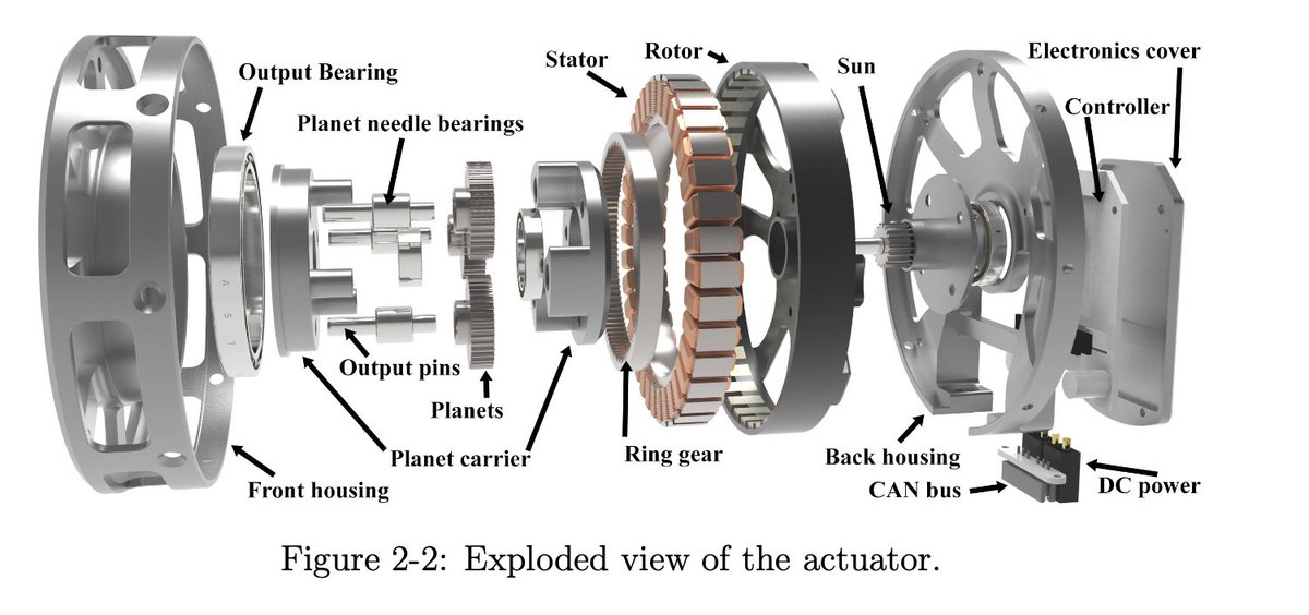
Figure 2.2: Exploded view of the MIT Mini Cheetah actuator module. Reproduced from Katz, Di Carlo, and Kim (2019).
Reading the exploded view front-to-back:
Front and back housing — the structural shell, with the output bearing supporting the load directly on the housing.
A single-stage planetary gear set — sun gear, planets on needle bearings, planet carrier, and ring gear. This is the entire gear reduction: one stage, giving the low ratio that Section 2.3.2 depends on.
A brushless motor — a stator (copper windings, held stationary) and a rotor (the ring of magnet poles around it). Note this is an outrunner layout: the magnets are on the outside, spinning around the fixed stator, which maximizes the radius the magnetic force acts at — and torque scales with that radius, so this geometry is a big part of how the motor gets its torque density without needing more gearing.
Back housing, controller, and connectors — the driver electronics (FOC current control) sit right behind the motor, with CAN bus and DC power connectors bringing both onto the same two-wire-plus-power interface described in Section 2.3.5.
The same architecture — housing, single planetary stage, outrunner BLDC, integrated FOC driver — is what today’s commercial QDD actuators (like the RobStride RS05 used for the concrete numbers below) build on.
2.3.4 Control Modes: MIT (Impedance) Mode and Beyond¶
The RobStride RS05 is a good concrete example of a modern, commercially available QDD actuator: 48 V rated (15–60 V range), a 7.75:1 single-stage planetary gearbox, a 20-pole outrunner BLDC motor driven by FOC, and CAN bus communication — the same architecture as the Mini Cheetah module above.
| Parameter | Value |
|---|---|
| Rated voltage | 48 V (15–60 V range) |
| Rated (continuous) torque | 1.6 N·m |
| Rated speed | 100 RPM |
| No-load speed | 480 RPM |
| Peak torque | 5.5 N·m |
| Peak phase current | 11 A (rated: 2.4 A) |
| Torque constant | 0.94 N·m/A |
| Gear ratio | 7.75:1 |
| Weight | 191 g |
| Communication | CAN 2.0, 1 Mbps |
The default control interface — what the datasheet calls operation control mode, active by default at power-on — is exactly the impedance/“MIT mode” idea this actuator class is known for. A single CAN frame carries five numbers — target position , target velocity , , , and a feedforward torque — and the actuator computes
entirely onboard, converting to a current command through its internal current loop. All five parameters pack into one 8-byte CAN data frame, so a full impedance command round-trips in a single packet.
This one equation covers a surprising range of behaviors, straight from the manual’s own worked examples:
Pure velocity control: , , , rad/s — the joint spins at 1 rad/s if unloaded; increase to hold that speed against an external load.
Pure damping (“brake”) mode: , , — the joint resists being turned, with resistance increasing with . This is genuinely regenerative: an external force turning the motor generates electricity, and the supply needs to be able to absorb it or the bus can overvoltage.
Position (“virtual spring”) mode: rad, , — the joint moves to 5 rad and holds there like a spring; raising stiffens the spring, and damps it (drop to zero and the joint oscillates around the target instead of settling).
That last case is impedance control in miniature: the actuator behaves like a programmable spring-damper, not a rigid position-tracker — precisely the compliant behavior that makes running and jumping possible.
Beyond operation control mode, the RS05 also exposes simpler, single-purpose modes reachable by switching run_mode: current mode (command directly — pure open-loop torque), velocity mode (speed regulation with a current limit and acceleration ramp), and two position modes — PP (Profile Position: send a target once, and the actuator’s own trapezoidal motion planner handles the speed/acceleration ramp) and CSP (Cyclic Synchronous Position: no onboard planning — the external controller streams a fresh position setpoint every cycle, and the actuator just tracks it). CSP is the mode a whole-body controller would use to stream a joint trajectory at a high, steady rate.
The RS05 also supports switching its CAN-layer protocol between a private protocol (the default, described above), CANopen (for integration with standard industrial motion controllers), and a literal MIT protocol mode — direct compatibility with the original open-source Mini Cheetah controller software. That three-way support is a good sign of how far the MIT actuator interface has spread as a de facto standard across the QDD ecosystem, alongside similar actuators like Damiao’s.
2.3.5 Daisy-Chaining over CAN Bus¶
QDD actuators daisy-chain the same way the bus servos in Section 2.2 do — many actuators sharing one communication bus and one power rail — but over CAN instead of a half-duplex UART bus. Each RS05 is assigned a CAN ID (0–127), and CAN’s built-in multi-master arbitration lets any node transmit without a single controller having to poll each actuator in turn, which half-duplex UART requires.
Two practical differences from Section 2.2’s daisy-chaining are worth flagging:
Comms loss is more dangerous here. A bus servo left without new commands just holds its last commanded angle — safe by default. A QDD joint running operation control mode is a torque source: if it kept applying its last torque command after the bus goes quiet, that could be actively unsafe. The RS05 handles this with a configurable
CAN_TIMEOUT— if no command arrives within the set window, the actuator drops into a safe reset state rather than continuing to apply torque blindly.Bandwidth, not just power, becomes the bottleneck. Because operation control mode streams full impedance commands at a high, steady rate — not the occasional “go to this angle” a bus servo gets — a single 1 Mbps CAN bus has a real ceiling on how many actuators it can command at full rate. This is why legged robots with a dozen or more QDD actuators (a quadruped alone needs 12) often split them across several CAN buses rather than one shared bus, trading Section 2.2’s power-budget concern for a bandwidth-budget one.
Key Takeaways — Section 2.3
Direct drive (no gearbox) makes motor current a trustworthy, high-bandwidth proxy for output torque and keeps the joint backdrivable — but a motor big enough to be useful direct-drive is too heavy to put on a leg.
QDD keeps that transparency by using a low gear ratio (e.g. ~7.75:1, a single planetary stage) paired with a high torque-density outrunner BLDC motor — a middle ground between a pure direct-drive motor and a highly-geared bus servo (~345:1).
The defining QDD control interface is impedance (“MIT”) mode: one CAN packet carries , , , , , and the actuator computes onboard — letting a single equation act as a programmable position controller, velocity controller, damper, or spring.
QDD actuators daisy-chain over CAN bus, sharing power and signal like a bus servo chain — but with a comms-timeout safety fallback (since a torque source is dangerous to leave uncommanded) and a command-rate bandwidth limit in place of a simple power budget.