Chapter 4 gave us the homogeneous transformation matrix (HTM): one matrix that stores both the position and the orientation of a frame, and that chains frames together by plain matrix multiplication. This chapter turns that tool into a recipe that works for any serial robot arm:
Forward position kinematics: given the joint variables , find the pose (position and orientation) of the gripper, .
The recipe has three steps — set up frames, write one HTM per link, multiply — and we apply it to five robots of increasing complexity, ending with a real industrial arm (the UR5e) whose geometry comes straight from a MuJoCo model file.
| Section | Topic |
|---|---|
| 5.1 | The general HTM and the six basic HTMs |
| 5.2 | Composition of HTMs, and how a joint moves a frame |
| 5.3 | The three-step forward kinematics procedure |
| 5.4 | Example 1 — planar 2R arm |
| 5.5 | Example 2 — 3R spherical wrist |
| 5.6 | Example 3 — RPP cylindrical robot |
| 5.7 | Example 4 — SCARA robot |
| 5.8 | Example 5 — UR5e from a MuJoCo model |
| 5.9 | The FK Frame Animator and chapter summary |
Notation used in this chapter. is the pose of frame relative to frame : the subscript names the frame being described, the superscript names the reference frame. Joint variables are ; for a prismatic joint we usually write instead, to remind us it is a length.
import numpy as np
import matplotlib.pyplot as plt
import sympy as sp
import re
from ipywidgets import interact, FloatSlider, IntSlider
from IPython.display import display, Math
%matplotlib inline

np.set_printoptions(precision=4, suppress=True)
5.1 The General HTM and the Basic HTMs¶
5.1.1 Reading an HTM column by column¶
Every HTM has the same block structure. For frame described in frame :
| Column | Meaning |
|---|---|
| unit vector along , expressed in frame | |
| unit vector along , expressed in frame | |
| unit vector along , expressed in frame | |
| coordinates of the origin , expressed in frame |
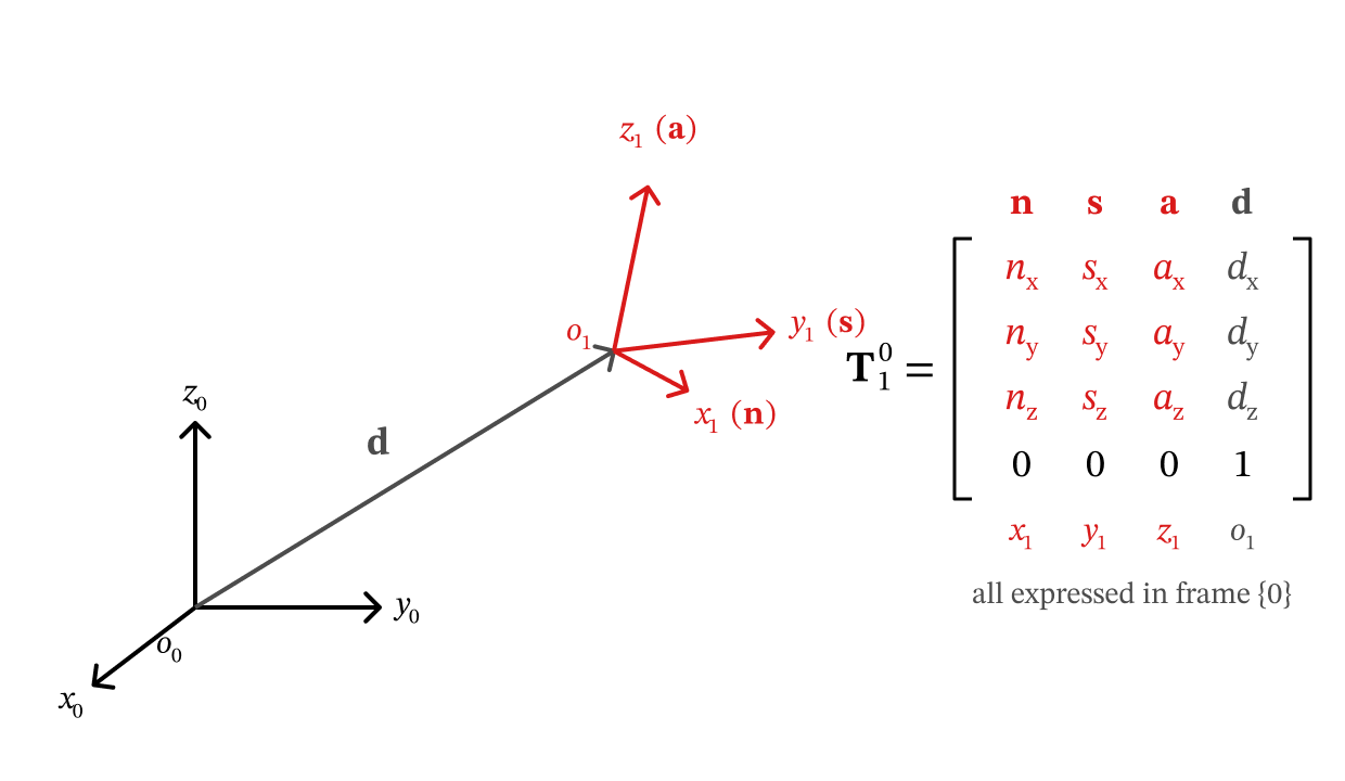
Figure 5.1 — The columns of T10 are the axes x1, y1, z1 (n, s, a) and the origin o1 (d), all written in frame {0}.
The first three columns form the rotation matrix (orientation); the last column is the position. So you can read a frame’s pose directly off its HTM: column 3 tells you where points, column 4 tells you where is.
5.1.2 The six basic HTMs¶
Almost every HTM we write in this chapter is a product of six basic HTMs: a pure translation along one axis, or a pure rotation about one axis.
Translation along , , by , , :
Rotation about , , by , , (with , , etc.):
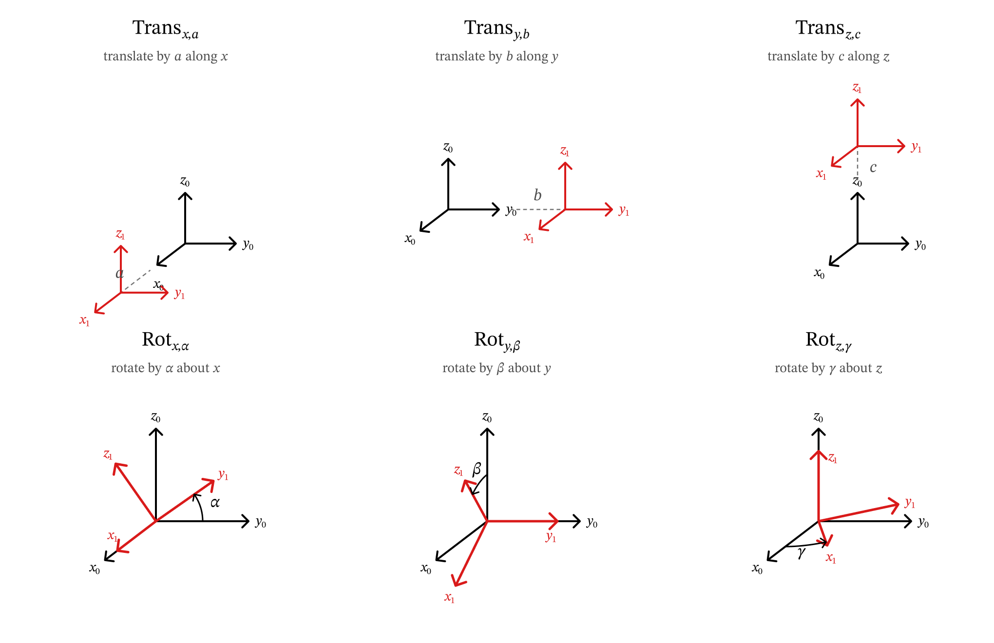
Figure 5.2 — The six basic HTMs: a pure translation along, or a pure rotation about, one axis.
A translation HTM has in the rotation block; a rotation HTM has the basic rotation matrix from Chapter 4 (, , ) in the rotation block and zero translation.
# ── The six basic HTMs ─────────────────────────────────────────────────────────

def Trans(axis, d):
    # Basic HTM: translate by d along the x, y or z axis.
    T = np.eye(4)
    T['xyz'.index(axis), 3] = d
    return T


def Rot(axis, theta):
    # Basic HTM: rotate by theta (radians) about the x, y or z axis.
    c, s = np.cos(theta), np.sin(theta)
    R = {'x': [[1, 0, 0], [0, c, -s], [0, s, c]],
         'y': [[c, 0, s], [0, 1, 0], [-s, 0, c]],
         'z': [[c, -s, 0], [s, c, 0], [0, 0, 1]]}[axis]
    T = np.eye(4)
    T[:3, :3] = R
    return T


def show(T, name='T'):
    # Print a 4x4 HTM with tidy rounding (no '-0.0').
    print(f'{name} =')
    print(np.round(T, 4) + 0.0)


show(Trans('y', 0.5), 'Trans_y,0.5')
print()
show(Rot('x', np.radians(90)), 'Rot_x,90°')
Trans_y,0.5 =
[[1. 0. 0. 0. ]
[0. 1. 0. 0.5]
[0. 0. 1. 0. ]
[0. 0. 0. 1. ]]
Rot_x,90° =
[[ 1. 0. 0. 0.]
[ 0. 0. -1. 0.]
[ 0. 1. 0. 0.]
[ 0. 0. 0. 1.]]
# ── Drawing helpers used throughout the chapter ────────────────────────────────

AXIS_COLORS = ('red', 'green', 'blue')          # x, y, z  (same as Chapter 4)


def draw_frame(ax, T, name='', scale=0.3, alpha=1.0, lw=2.0, axis_labels=True, stack=0):
    # Draw the frame whose pose in frame {0} is the HTM T.
    # stack > 0 shifts the {name} label down, for frames that share an origin.
    o = T[:3, 3]
    for i, col in enumerate(AXIS_COLORS):
        v = T[:3, i] * scale
        ax.quiver(*o, *v, color=col, alpha=alpha, linewidth=lw, arrow_length_ratio=0.2)
        if axis_labels and name and alpha >= 0.5:
            ax.text(*(o + 1.25 * v), f'${"xyz"[i]}_{{{name}}}$', color=col, fontsize=9)
    if name and alpha >= 0.5:
        ax.text(*(o - 0.25 * scale - np.array([0, 0, 0.6 * scale * stack])),
                f'{{{name}}}', fontsize=9, fontweight='bold')


def setup_3d(ax, center=(0, 0, 0), half=1.0, view=(25, -60), title='', zhalf=None):
    # Equal-scale 3D axes centred on `center`; zhalf (optional) shrinks the z-range.
    c = np.asarray(center, float)
    zh = half if zhalf is None else zhalf
    ax.set_xlim(c[0] - half, c[0] + half)
    ax.set_ylim(c[1] - half, c[1] + half)
    ax.set_zlim(c[2] - zh, c[2] + zh)
    ax.set_box_aspect((1, 1, zh / half))
    ax.set_xlabel('$x_0$'); ax.set_ylabel('$y_0$'); ax.set_zlabel('$z_0$')
    ax.view_init(*view)
    if title:
        ax.set_title(title, fontsize=11)


# ── Picture of the six basic HTMs acting on frame {0} ──────────────────────────
basics = [(Trans('x', 0.6), r'$\mathrm{Trans}_{x,0.6}$'),
          (Trans('y', 0.6), r'$\mathrm{Trans}_{y,0.6}$'),
          (Trans('z', 0.6), r'$\mathrm{Trans}_{z,0.6}$'),
          (Rot('x', np.radians(60)), r'$\mathrm{Rot}_{x,60^\circ}$'),
          (Rot('y', np.radians(60)), r'$\mathrm{Rot}_{y,60^\circ}$'),
          (Rot('z', np.radians(60)), r'$\mathrm{Rot}_{z,60^\circ}$')]

fig = plt.figure(figsize=(13, 8))
for i, (T, title) in enumerate(basics):
    ax = fig.add_subplot(2, 3, i + 1, projection='3d')
    draw_frame(ax, np.eye(4), '0', scale=0.6, alpha=0.25)
    draw_frame(ax, T, '1', scale=0.6)
    setup_3d(ax, center=(0.25, 0.25, 0.25), half=0.75, title=title)
fig.suptitle('The six basic HTMs: faded = frame {0}, solid = frame {1} with $T_1^0$ = the basic HTM',
             fontsize=12)
plt.tight_layout(); plt.show()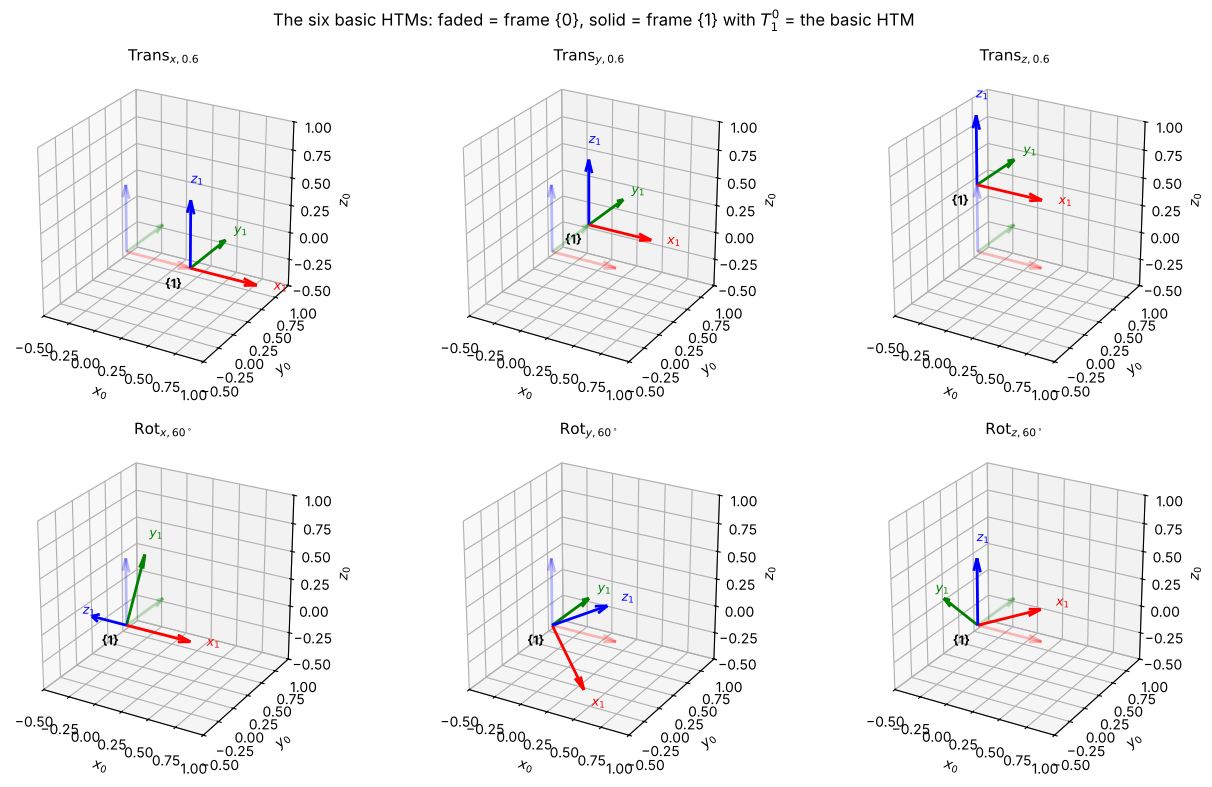
Key Takeaways — Section 5.1
The columns of are the , , unit vectors and the origin , all expressed in frame .
Six basic HTMs — , , , , , — are the building blocks for every HTM in this chapter.
5.2 Composition of HTMs, and How a Joint Moves a Frame¶
5.2.1 Composition¶
If we know frame relative to and frame relative to , then
The inner indices match and “cancel” ( appears once as a subscript and once as a superscript), which is an easy way to check that a product is written in the right order.
5.2.2 Reading a product of basic HTMs¶
A product of basic HTMs can be read left to right as a sequence of moves of a frame, where every move is made along or about the frame’s current axes (this is the post-multiplication / body-axis rule from Chapter 4, §4.3.2). For example
means: start at frame , slide 1 along , then rotate about the new , then rotate about the newest . Where the frame ends up is frame .
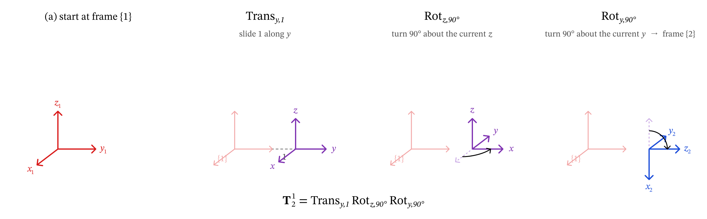
Figure 5.3 — Reading T21 = Transy,1 Rotz,90° Roty,90° left to right: each move uses the frame’s current axes.
5.2.3 Worked example (Lecture 8)¶
Frame sits 1 unit above the ground frame with the same orientation, and frame is obtained from frame by the three moves above:
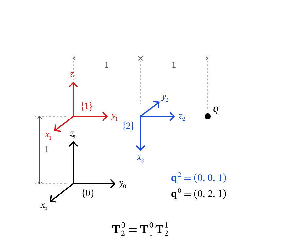
Figure 5.4 — Lecture 8 example: frame {1} is 1 above {0}; frame {2} is reached by the moves of Figure 5.3; q is 1 along z2.
A point sits 1 unit along : . Where is it in frame ? Augment with a 1 and multiply:
T10 = Trans('z', 1)
T21 = Trans('y', 1) @ Rot('z', np.radians(90)) @ Rot('y', np.radians(90))
T20 = T10 @ T21                          # composition: inner indices '1' cancel

show(T21, 'T_2^1')
print()
show(T20, 'T_2^0')

q2 = np.array([0, 0, 1, 1])              # q in frame {2}, augmented with a 1
q1 = T21 @ q2
q0 = T20 @ q2
print('\nq^2 =', q2[:3], '  q^1 =', q1[:3], '  q^0 =', q0[:3])
print('Matches the lecture result q^0 = (0, 2, 1)?', np.allclose(q0[:3], [0, 2, 1]))
T_2^1 =
[[ 0. -1. 0. 0.]
[ 0. 0. 1. 1.]
[-1. 0. 0. 0.]
[ 0. 0. 0. 1.]]
T_2^0 =
[[ 0. -1. 0. 0.]
[ 0. 0. 1. 1.]
[-1. 0. 0. 1.]
[ 0. 0. 0. 1.]]
q^2 = [0 0 1] q^1 = [0. 2. 0.] q^0 = [0. 2. 1.]
Matches the lecture result q^0 = (0, 2, 1)? True
Below, the slider applies the factors of one at a time. The bold frame with a black dot is the moving frame after the factors applied so far; faded frames are earlier intermediate stops, and a labeled frame appears each time a is complete. Watch how each rotation acts about the moving frame’s current axis.
The two helper functions in the next cell are reused for every robot in this chapter. A product is stored as a list of groups — one group per — and each group is a list of basic-HTM factors.
# ── Factors and chains: a product of basic HTMs, stored so we can step through it ─

def Tr(axis, val, tex):
    # One translation factor; tex is the LaTeX for the amount, e.g. 'L_1'.
    return dict(kind='trans', axis=axis, val=val, tex=rf'\mathrm{{Trans}}_{{{axis},{tex}}}')


def Rt(axis, val, tex):
    # One rotation factor (val in radians); tex is the LaTeX for the angle.
    return dict(kind='rot', axis=axis, val=val, tex=rf'\mathrm{{Rot}}_{{{axis},{tex}}}')


def factor_T(f):
    return Trans(f['axis'], f['val']) if f['kind'] == 'trans' else Rot(f['axis'], f['val'])


def chain_frames(groups):
    # groups = [(frame name, [factors]), ...]  ->  {frame name: T^0 of that frame}
    T, frames = np.eye(4), {'0': np.eye(4)}
    for name, factors in groups:
        for f in factors:
            T = T @ factor_T(f)
        frames[name] = T
    return frames


def product_latex(groups, k, lhs):
    # LaTeX for the whole product, with the factors not yet applied shown in grey.
    out, j = [], 0
    for _, factors in groups:
        for f in factors:
            out.append(f['tex'] if j < k else r'{\color{lightgray}' + f['tex'] + '}')
            j += 1
    return lhs + ' = ' + r'\,'.join(out)


def plot_chain(ax, groups, k=None, scale=0.25, skeleton=True, axis_labels=True, **setup_kw):
    # Draw the frames of a chain. If k is given, show only the first k factors applied
    # (faded frames = intermediate stops, black dot = the moving frame).
    flat = [(name, f) for name, factors in groups for f in factors]
    N = len(flat)
    k = N if k is None else k
    ends = np.cumsum([len(fs) for _, fs in groups])       # factor count at each frame
    names = [name for name, _ in groups]

    if skeleton:                                           # links: polyline through origins
        pts = np.array([T[:3, 3] for T in chain_frames(groups).values()])
        ax.plot(*pts.T, color='0.5', lw=6, alpha=1.0 if k == N else 0.25,
                solid_capstyle='round', zorder=0)
        ax.scatter(*pts[:-1].T, color='0.25', s=40, alpha=1.0 if k == N else 0.25)

    seen = {}                                              # frames sharing an origin

    def n_before(T):
        key = tuple(np.round(T[:3, 3], 3))
        seen[key] = seen.get(key, -1) + 1
        return seen[key]

    draw_frame(ax, np.eye(4), '0', scale=scale * 1.3, axis_labels=axis_labels, stack=n_before(np.eye(4)))
    T = np.eye(4)
    for j in range(k):
        T = T @ factor_T(flat[j][1])
        if j + 1 in ends:                                   # a T_i^{i-1} is complete
            n = n_before(T)                                 # shorter arrows if origin is shared
            draw_frame(ax, T, names[list(ends).index(j + 1)], scale=scale * max(0.55, 1 - 0.15 * n),
                       axis_labels=axis_labels, stack=n)
        elif j == k - 1:                                    # the moving frame right now: bold
            draw_frame(ax, T, scale=scale, lw=3)
        else:                                               # an earlier intermediate stop: faded
            draw_frame(ax, T, scale=scale * 0.8, alpha=0.3, lw=1)
    if k < N:                                               # mark the moving frame
        ax.scatter(*T[:3, 3], color='black', s=25, zorder=5)
    setup_3d(ax, **setup_kw)
    return T, N


# ── Step through the Lecture 8 example ─────────────────────────────────────────
groups_L8 = [('1', [Tr('z', 1, '1')]),
             ('2', [Tr('y', 1, '1'), Rt('z', np.pi / 2, r'90^\circ'), Rt('y', np.pi / 2, r'90^\circ')])]


def step_L8(k):
    fig = plt.figure(figsize=(6.5, 6))
    ax = fig.add_subplot(111, projection='3d')
    T, N = plot_chain(ax, groups_L8, k, scale=0.35, center=(0, 0.6, 0.6), half=1.0)
    q0 = (chain_frames(groups_L8)['2'] @ np.array([0, 0, 1, 1]))[:3]
    if k == N:
        ax.scatter(*q0, color='purple', s=60)
        ax.text(*(q0 + 0.08), '$q$', color='purple', fontsize=12)
    plt.show()
    display(Math(product_latex(groups_L8, k, r'\mathbf{T}_2^0')))
    show(T, f'Product of the first {k} factor(s)')


interact(step_L8, k=IntSlider(value=4, min=0, max=4, description='factors'));5.2.4 How a joint moves a frame (Lecture 8)¶
Now attach frame to a link that turns on a revolute joint whose axis is . At the home configuration () the frame is . When the joint turns by , the link — and the frame glued to it — rotates about the joint axis to a new frame :
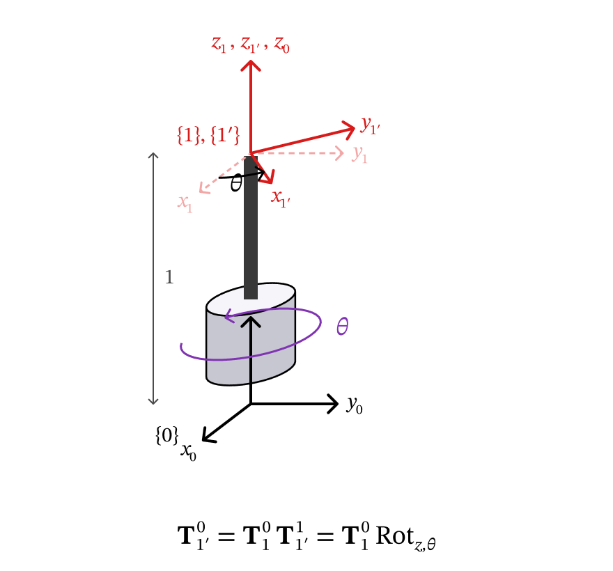
Figure 5.5 — A revolute joint about z1 turns frame {1} into {1′}: post-multiply by Rotz,θ.
This only works as a single post-multiplied because we chose to lie along the joint axis: rotating about the joint axis is then the same as rotating about the frame’s own current -axis. That choice is the key idea of the whole procedure in Section 5.3.
Key Takeaways — Section 5.2
Compose frames by multiplying HTMs: (inner indices cancel).
Read a product of basic HTMs left to right: each factor moves the frame along or about its current axes.
Augment a point with a 1 to transform it: .
If lies along joint ’s axis, turning the joint by just post-multiplies the frame by .
5.3 The Forward Kinematics Procedure¶
For an -joint robotic arm:
Step 1 — Set up a frame for each link.
Frame : fixed to the ground (the inertial frame).
Frames : frame is fixed to link and moves with joint . Put along the axis of joint (the rotation axis for a revolute joint, the sliding direction for a prismatic joint).
Frame : at the gripper (end-effector) center. Because there is no joint between frame and frame , is constant.
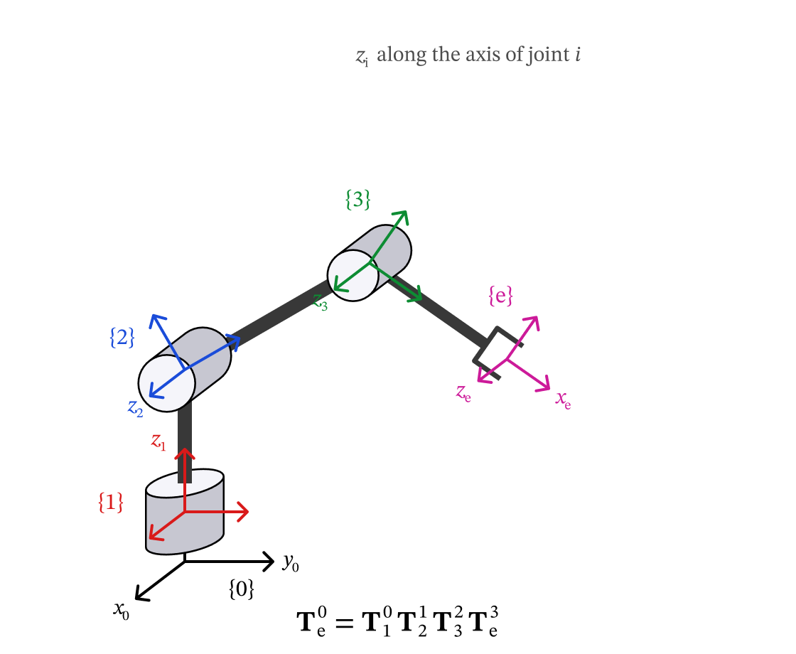
Figure 5.6 — Step 1: frame {0} on the ground, frame {i} on link i with zi along joint i, frame {e} at the gripper.
Step 2 — Obtain for .
Home configuration ( for all ): write as a product of basic HTMs that moves frame onto frame .
Joint motion (): post-multiply by one basic HTM along/about :
Step 3 — Multiply.
The position of the gripper is the last column of ; its orientation is the upper-left block.
Note for readers of other textbooks. Many books use the Denavit–Hartenberg (DH) convention, which restricts how frames may be placed so that each link needs exactly four parameters. Our procedure lets you place frames freely (only along joint is required) and writes with any basic HTMs you like. Both give the same ; ours is easier to set up from a drawing or a CAD/MJCF model.
The class below is a direct translation of Steps 2 and 3 into code. Each example in this chapter only has to supply the home factors of every , the joint types, and the constant tool factors of .
class Robot:
    # A serial arm described by the three-step FK procedure.
    #   home   : home[i] = list of factors whose product is T_{i+1}^{i}(0)
    #   joints : list of (slider label, LaTeX symbol, 'R' or 'P', (min, max))
    #   tool   : list of factors whose product is the constant T_e^n

    def __init__(self, name, home, joints, tool):
        self.name, self.home, self.joints, self.tool = name, home, joints, tool

    def groups(self, q):
        # Step 2: T_i^{i-1}(q_i) = T_i^{i-1}(0) * Rot_z,q_i  (or Trans_z,q_i)
        G = []
        for i, (_, tex, jtype, _) in enumerate(self.joints):
            motion = Rt('z', q[i], tex) if jtype == 'R' else Tr('z', q[i], tex)
            G.append((str(i + 1), self.home[i] + [motion]))
        G.append(('e', self.tool))
        return G

    def frames(self, q):
        return chain_frames(self.groups(q))       # every frame's T^0

    def fk(self, q):
        return self.frames(q)['e']                 # Step 3: T_e^0


def explore(robot, figsize=(7, 6.5), **setup_kw):
    # Interactive view: one slider per joint, plus a slider that steps through the product.
    sliders = {}
    for i, (label, _, jtype, (lo, hi)) in enumerate(robot.joints):
        unit = ' (°)' if jtype == 'R' else ''
        sliders[f'q{i}'] = FloatSlider(value=0, min=lo, max=hi, step=1 if jtype == 'R' else 0.01,
                                      description=label + unit)
    N = sum(len(fs) for _, fs in robot.groups(np.zeros(len(robot.joints))))
    sliders['k'] = IntSlider(value=N, min=0, max=N, description='factors')

    def _view(k, **qs):
        q = [np.radians(qs[f'q{i}']) if j[2] == 'R' else qs[f'q{i}']
             for i, j in enumerate(robot.joints)]
        G = robot.groups(q)
        fig = plt.figure(figsize=figsize)
        ax = fig.add_subplot(111, projection='3d')
        T, _ = plot_chain(ax, G, k, title=robot.name, **setup_kw)
        plt.show()
        display(Math(product_latex(G, k, r'\mathbf{T}_e^0')))
        show(T, 'T_e^0' if k == N else f'Product of the first {k} factor(s)')

    interact(_view, **sliders)


def snapshot(robot, poses, titles, figsize=(13, 5.5), **setup_kw):
    # Static side-by-side pictures of the robot at a few joint vectors (radians / metres).
    fig = plt.figure(figsize=figsize)
    for i, (q, t) in enumerate(zip(poses, titles)):
        ax = fig.add_subplot(1, len(poses), i + 1, projection='3d')
        plot_chain(ax, robot.groups(q), title=t, **setup_kw)
    plt.tight_layout(); plt.show()
# ── SymPy versions of the basic HTMs, for closed-form FK ───────────────────────
def sTrans(axis, d):
T = sp.eye(4)
T['xyz'.index(axis), 3] = d
return T
def sRot(axis, t):
c, s = sp.cos(t), sp.sin(t)
R = {'x': [[1, 0, 0], [0, c, -s], [0, s, c]],
'y': [[c, 0, s], [0, 1, 0], [-s, 0, c]],
'z': [[c, -s, 0], [s, c, 0], [0, 0, 1]]}[axis]
T = sp.eye(4)
T[:3, :3] = sp.Matrix(R)
return T
def show_sym(T, lhs):
# Display a symbolic matrix using the shorthand c_1 = cos(theta_1), s_12 = sin(theta_1+theta_2), ...
tex = sp.latex(T)
def short(m):
fn, inner = m.group(1), m.group(2)
idx = re.findall(r'\\theta_\{(\d)\}', inner)
rest = re.sub(r'\\theta_\{\d\}|\+|\s', '', inner)
return f'{fn[0]}_{{{"".join(idx)}}}' if idx and not rest else m.group(0)
tex = re.sub(r'\\(cos|sin)\{\\left\((.*?)\\right\)\}', short, tex)
display(Math(lhs + ' = ' + tex))Key Takeaways — Section 5.3
Step 1: frame on the ground, frame on link with along joint , frame at the gripper.
Step 2: write the home transform from basic HTMs, then post-multiply by (revolute) or (prismatic).
Step 3: .
The same three steps work for any serial robot, from a 2R arm to a 6-DOF industrial arm.
5.4 Example 1 — Planar 2R Arm¶
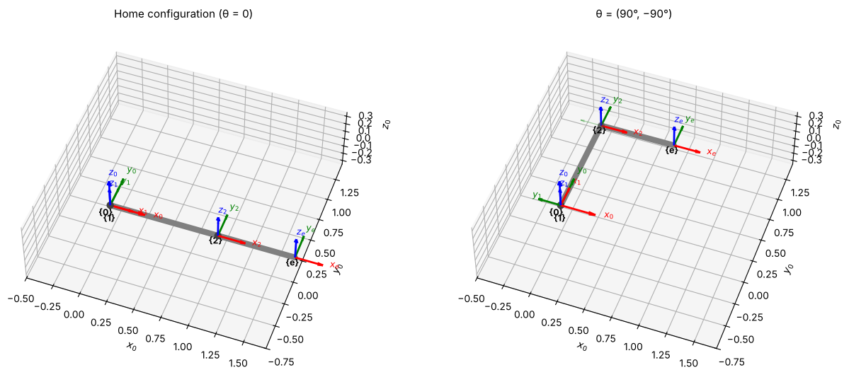
Two revolute joints with parallel axes (out of the page), link lengths and . This is the Chapter 3 robot, so we already know the answer — a good first test of the procedure.
Step 1 — Frames. All -axes point out of the page (along the joint axes). At home the arm is stretched along : frame coincides with , frame is at the elbow, frame at the tip. All frames stay parallel at home.
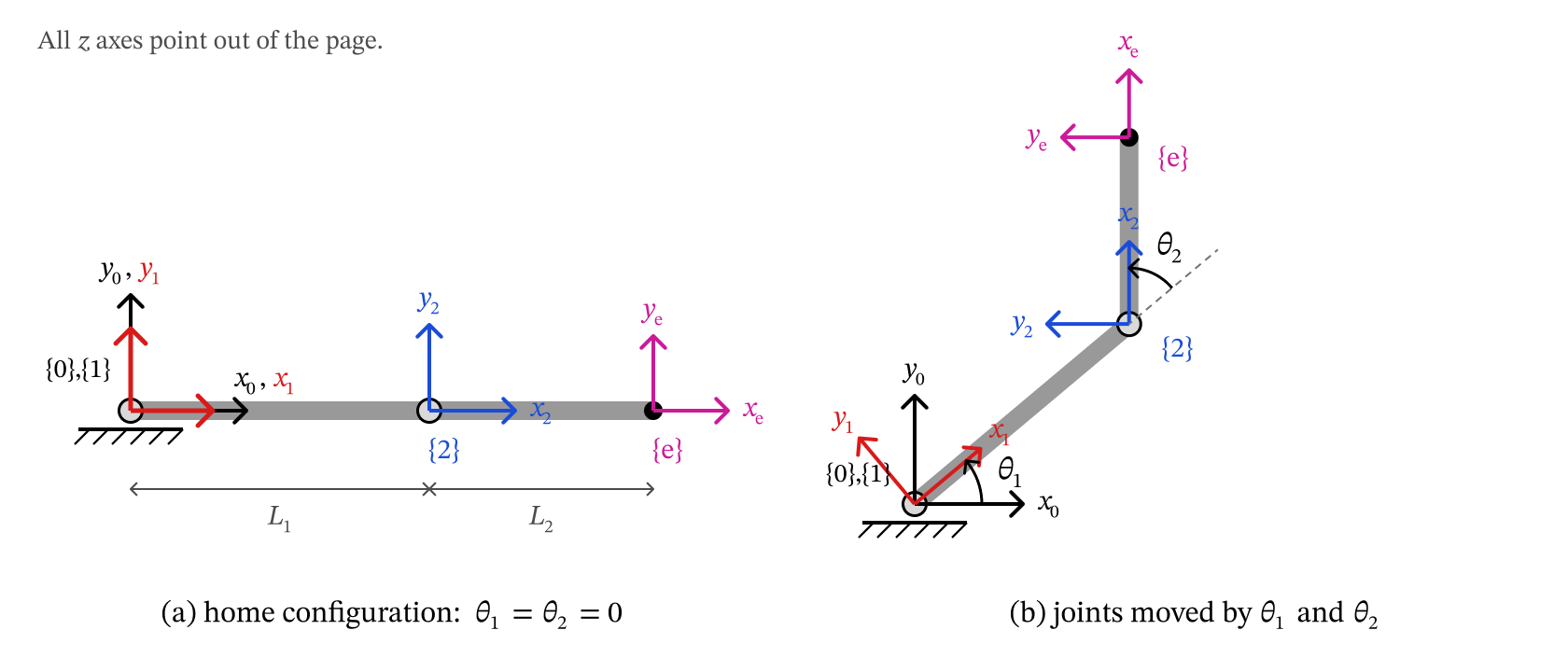
Figure 5.7 — Example 1 (Lecture 9): frames of the planar 2R arm at home (a) and after the joints move (b).
Step 2 — Home configuration and joint motion.
Step 3 — Multiply.
Read it left to right: turn by , walk , turn by , walk .
L1, L2 = 1.0, 0.7


def fk_2R(th1, th2, L1=1.0, L2=0.7):
    # Step 2 — home configuration (θ = 0)
    T10_0 = np.eye(4)                       # T_1^0(0)
    T21_0 = Trans('x', L1)                  # T_2^1(0)
    Te2   = Trans('x', L2)                  # T_e^2 (constant)
    # Step 2 — joint motion
    T10 = T10_0 @ Rot('z', th1)             # revolute joint 1
    T21 = T21_0 @ Rot('z', th2)             # revolute joint 2
    # Step 3
    return T10 @ T21 @ Te2


th1, th2 = np.radians(90), np.radians(-90)
Te0 = fk_2R(th1, th2)
show(Te0, 'T_e^0 at (θ1, θ2) = (90°, -90°)')

# Compare with the Chapter 3 trigonometry
x = L1*np.cos(th1) + L2*np.cos(th1 + th2)
y = L1*np.sin(th1) + L2*np.sin(th1 + th2)
print(f'\nChapter 3 formula: (x, y) = ({x:.4f}, {y:.4f})   matches column 4? {np.allclose(Te0[:2, 3], [x, y])}')
T_e^0 at (θ1, θ2) = (90°, -90°) =
[[1. 0. 0. 0.7]
[0. 1. 0. 1. ]
[0. 0. 1. 0. ]
[0. 0. 0. 1. ]]
Chapter 3 formula: (x, y) = (0.7000, 1.0000) matches column 4? True
# Closed form with SymPy
t1, t2, l1, l2 = sp.symbols('theta_1 theta_2 L_1 L_2', real=True)
Te0_2R = sp.simplify(sRot('z', t1) * sTrans('x', l1) * sRot('z', t2) * sTrans('x', l2))
show_sym(Te0_2R, r'\mathbf{T}_e^0')with , , , . The last column is exactly the Chapter 3 result , — and we get the orientation (a rotation of about ) for free.
robot_2R = Robot('Example 1: planar 2R',
                 home=[[], [Tr('x', L1, 'L_1')]],
                 joints=[('θ₁', r'\theta_1', 'R', (-180, 180)),
                         ('θ₂', r'\theta_2', 'R', (-180, 180))],
                 tool=[Tr('x', L2, 'L_2')])

view_2R = dict(center=(0.6, 0.35, 0), half=1.1, zhalf=0.35, view=(50, -70))

# Generic Robot class agrees with the hand-written fk_2R?
q_test = np.radians([37, -112])
print('Robot.fk matches fk_2R:', np.allclose(robot_2R.fk(q_test), fk_2R(*q_test)))

snapshot(robot_2R, [np.zeros(2), np.radians([90, -90])],
         ['Home configuration (θ = 0)', 'θ = (90°, −90°)'], **view_2R)
Robot.fk matches fk_2R: True
explore(robot_2R, **view_2R)Key Takeaways — Section 5.4
: “turn, walk, turn, walk”.
The position column reproduces the Chapter 3 formula; the rotation block adds the orientation .
5.5 Example 2 — 3R Spherical Wrist¶
Three revolute joints whose axes all meet at one point (the wrist center): roll, pitch, roll. A gripper sits a distance beyond the wrist center along the last axis.
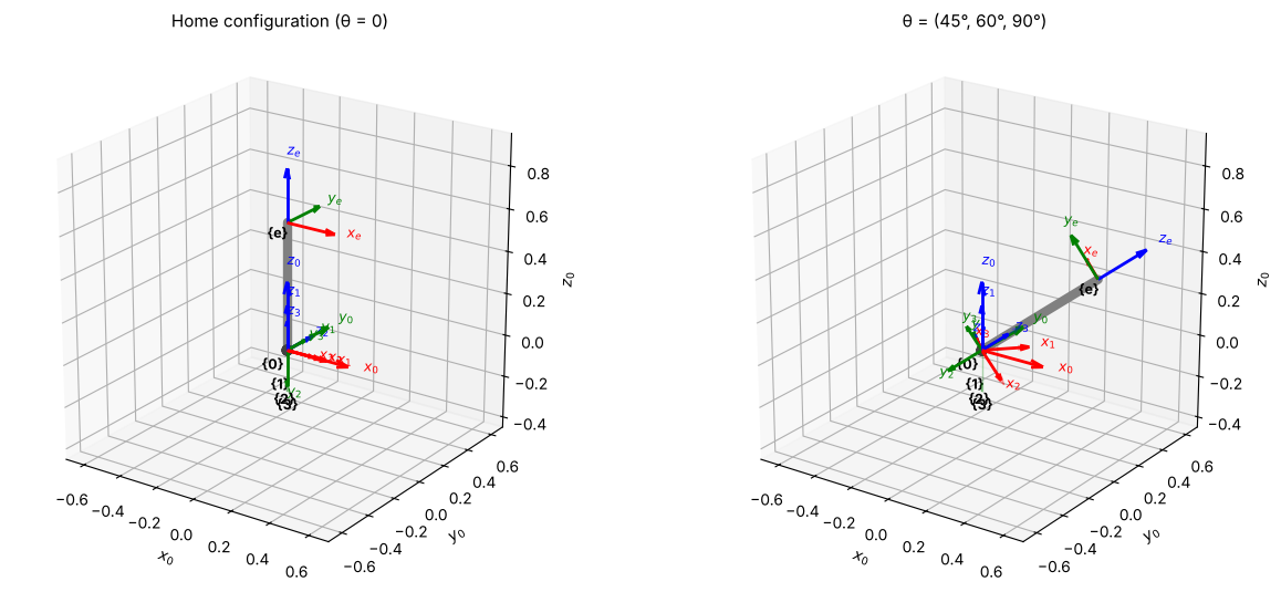
Step 1 — Frames. Put every along joint . Because the axes intersect, all three origins are at the wrist center: . At home, and point up (along ) and points along , the pitch axis.
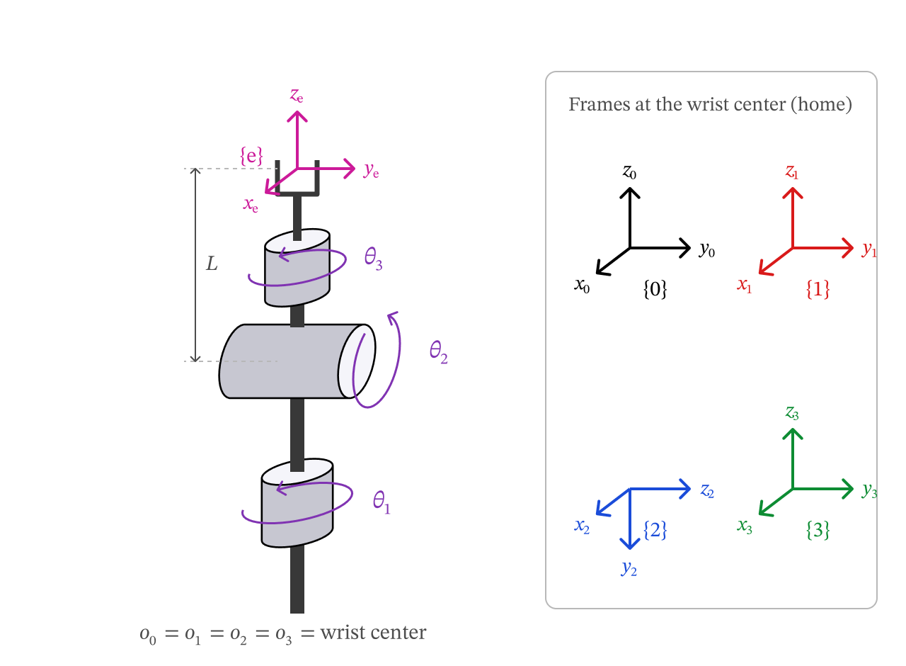
Figure 5.8 — Example 2 (Lecture 9): the spherical wrist. All joint axes meet at the wrist center.
Step 2 — Home configuration and joint motion.
tips over so that lies along the pitch axis, and tips it back up for the third (roll) joint. Then
Step 3 — Multiply.
L = 0.6


def fk_wrist(th1, th2, th3, L=0.6):
    # Step 2 — home configuration (θ = 0)
    T10_0 = np.eye(4)                       # T_1^0(0)
    T21_0 = Rot('x', np.radians(-90))       # T_2^1(0)
    T32_0 = Rot('x', np.radians(90))        # T_3^2(0)
    Te3   = Trans('z', L)                   # T_e^3 (constant)
    # Step 2 — joint motion (all revolute)
    T10 = T10_0 @ Rot('z', th1)
    T21 = T21_0 @ Rot('z', th2)
    T32 = T32_0 @ Rot('z', th3)
    # Step 3
    return T10 @ T21 @ T32 @ Te3


show(fk_wrist(0, np.radians(90), 0), 'T_e^0 at (θ1, θ2, θ3) = (0, 90°, 0)')
T_e^0 at (θ1, θ2, θ3) = (0, 90°, 0) =
[[ 0. 0. 1. 0.6]
[ 0. 1. 0. 0. ]
[-1. 0. 0. 0. ]
[ 0. 0. 0. 1. ]]
t1, t2, t3, Ls = sp.symbols('theta_1 theta_2 theta_3 L', real=True)
Te0_wrist = sp.simplify(sRot('z', t1) * sRot('x', -sp.pi/2) * sRot('z', t2)
                        * sRot('x', sp.pi/2) * sRot('z', t3) * sTrans('z', Ls))
show_sym(Te0_wrist, r'\mathbf{T}_e^0')

# The middle three factors are just a rotation about y:
middle = sp.simplify(sRot('x', -sp.pi/2) * sRot('z', t2) * sRot('x', sp.pi/2))
print('Rot_x,-90 · Rot_z,θ2 · Rot_x,90 == Rot_y,θ2 ?', sp.simplify(middle - sRot('y', t2)) == sp.zeros(4))Rot_x,-90 · Rot_z,θ2 · Rot_x,90 == Rot_y,θ2 ? True
Two things to notice:
The gripper position is — a point on a sphere of radius , which is why this is called a spherical wrist. does not move the gripper’s position at all; it only spins the gripper about its own axis.
, so the orientation is — exactly the ZYZ Euler angles. A spherical wrist can reach any orientation, which is why most 6-DOF arms end with one.
robot_wrist = Robot('Example 2: spherical wrist (roll–pitch–roll)',
                    home=[[], [Rt('x', -np.pi/2, r'-90^\circ')], [Rt('x', np.pi/2, r'90^\circ')]],
                    joints=[('θ₁', r'\theta_1', 'R', (-180, 180)),
                            ('θ₂', r'\theta_2', 'R', (-180, 180)),
                            ('θ₃', r'\theta_3', 'R', (-180, 180))],
                    tool=[Tr('z', L, 'L')])

view_wrist = dict(center=(0, 0, 0.25), half=0.7, view=(22, -55))
q_test = np.radians([20, -50, 75])
print('Robot.fk matches fk_wrist:', np.allclose(robot_wrist.fk(q_test), fk_wrist(*q_test)))

snapshot(robot_wrist, [np.zeros(3), np.radians([45, 60, 90])],
         ['Home configuration (θ = 0)', 'θ = (45°, 60°, 90°)'], **view_wrist)
Robot.fk matches fk_wrist: True
explore(robot_wrist, **view_wrist)Key Takeaways — Section 5.5
When joint axes intersect, several frames share one origin; the home transforms are then pure rotations.
Fixed rotations in (here ) exist only to point along joint .
Spherical wrist: position , orientation (ZYZ Euler angles).
5.6 Example 3 — RPP Cylindrical Robot¶
A revolute base , a prismatic vertical lift , and a prismatic horizontal reach . The shoulder is at height and the reach slide starts a distance from the column.
Step 1 — Frames. along the base axis (up). along the lift direction (up), at height . along the reach direction, which at home is ; the gripper is at the end of the reach slide, so frame coincides with frame .
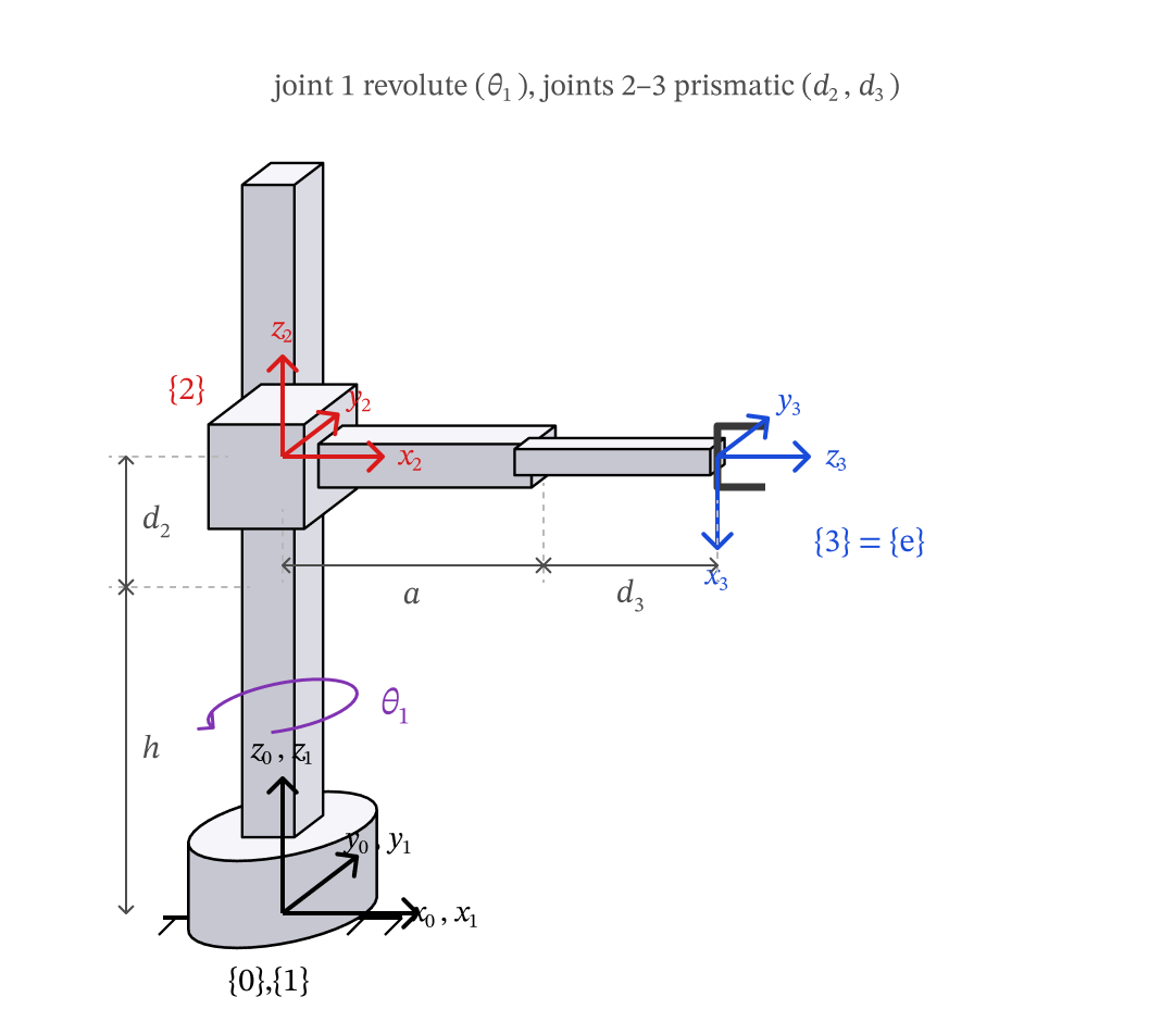
Figure 5.9 — Example 3: the RPP cylindrical robot, with base height h, lift d2, offset a and reach d3.
Step 2 — Home configuration and joint motion.
turns to point along the old so that lies along the reach slide. Joints 2 and 3 are prismatic, so they post-multiply by :
Step 3 — Multiply.
h, a = 0.8, 0.7


def fk_rpp(th1, d2, d3, h=0.8, a=0.7):
    # Step 2 — home configuration (θ1 = d2 = d3 = 0)
    T10_0 = np.eye(4)                                   # T_1^0(0)
    T21_0 = Trans('z', h)                               # T_2^1(0)
    T32_0 = Trans('x', a) @ Rot('y', np.radians(90))    # T_3^2(0)
    Te3   = np.eye(4)                                   # T_e^3: frame e = frame 3
    # Step 2 — joint motion
    T10 = T10_0 @ Rot('z', th1)             # revolute
    T21 = T21_0 @ Trans('z', d2)            # prismatic
    T32 = T32_0 @ Trans('z', d3)            # prismatic
    # Step 3
    return T10 @ T21 @ T32 @ Te3


show(fk_rpp(np.radians(90), 0, 0), 'T_e^0 at (θ1, d2, d3) = (90°, 0, 0)')
T_e^0 at (θ1, d2, d3) = (90°, 0, 0) =
[[ 0. -1. 0. 0. ]
[ 0. 0. 1. 0.7]
[-1. 0. 0. 0.8]
[ 0. 0. 0. 1. ]]
t1, d2, d3, hs, as_ = sp.symbols('theta_1 d_2 d_3 h a', real=True)
Te0_rpp = sp.simplify(sRot('z', t1) * sTrans('z', hs) * sTrans('z', d2)
                      * sTrans('x', as_) * sRot('y', sp.pi/2) * sTrans('z', d3))
show_sym(Te0_rpp, r'\mathbf{T}_e^0')The gripper position is exactly cylindrical coordinates: radius , angle , height — hence the name. Notice the prismatic variables enter the position linearly, while the revolute variable enters through and .
robot_rpp = Robot('Example 3: RPP cylindrical robot',
                  home=[[], [Tr('z', h, 'h')], [Tr('x', a, 'a'), Rt('y', np.pi/2, r'90^\circ')]],
                  joints=[('θ₁', r'\theta_1', 'R', (-180, 180)),
                          ('d₂', 'd_2', 'P', (-0.4, 0.5)),
                          ('d₃', 'd_3', 'P', (-0.3, 0.5))],
                  tool=[])

view_rpp = dict(center=(0.3, 0.1, 0.6), half=0.9, view=(22, -60))
q_test = [np.radians(-35), 0.2, 0.3]
print('Robot.fk matches fk_rpp:', np.allclose(robot_rpp.fk(q_test), fk_rpp(*q_test)))

snapshot(robot_rpp, [np.zeros(3), [np.radians(90), 0.3, 0.4]],
         ['Home configuration', 'θ₁ = 90°, d₂ = 0.3, d₃ = 0.4'], **view_rpp)
Robot.fk matches fk_rpp: True
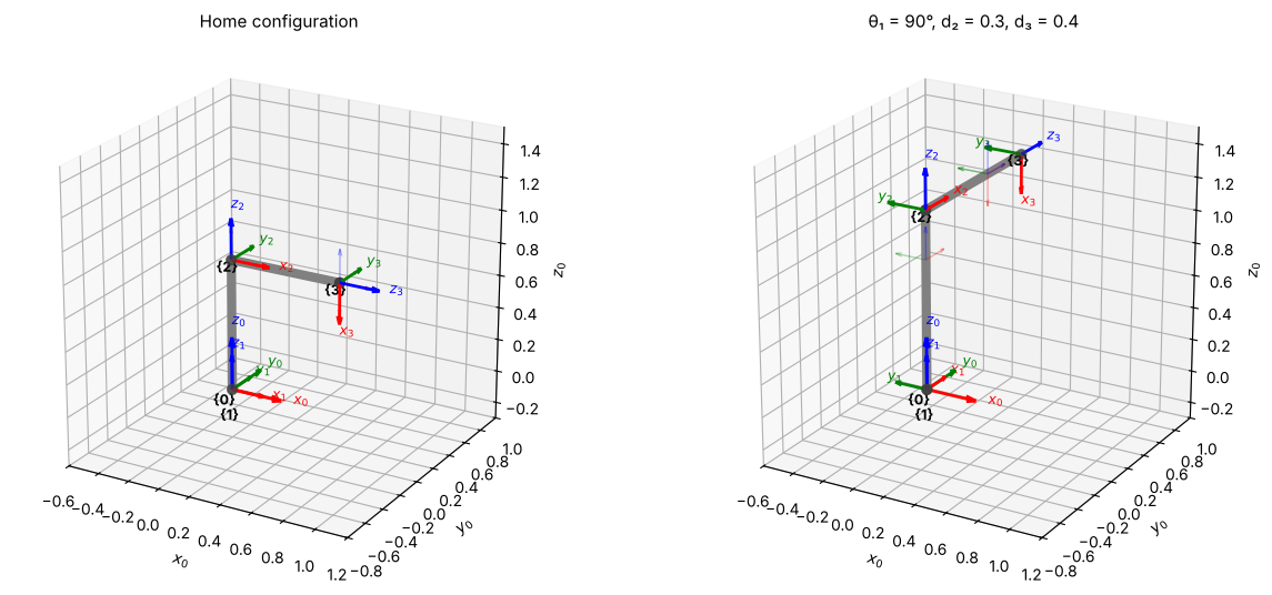
explore(robot_rpp, **view_rpp)Key Takeaways — Section 5.6
A prismatic joint post-multiplies by instead of — that is the only change.
If no tool offset is needed, frame can coincide with frame : .
RPP robot: — cylindrical coordinates.
5.7 Example 4 — SCARA Robot (RRPR)¶
The SCARA (Selective Compliance Assembly Robot Arm) is the standard pick-and-place robot: two vertical revolute joints (, ) move the arm in a horizontal plane, a prismatic quill () moves the tool down, and a final revolute joint () rolls the tool. Parameters: shoulder height , link lengths , , and tool length .
Step 1 — Frames. and point up along the two vertical revolute axes. The quill moves downward, so we flip the frame with : and point down. Frame is at the tool tip, further along .
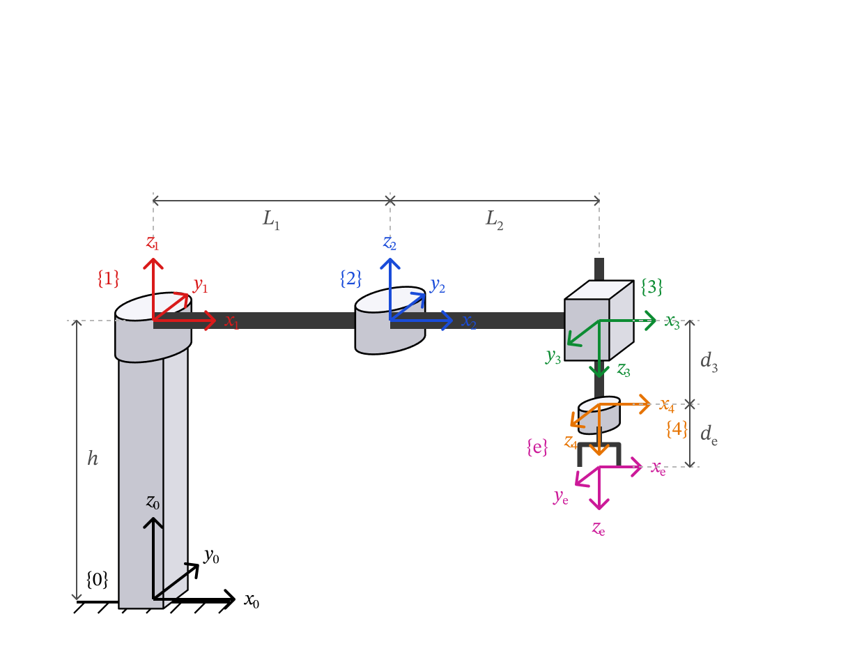
Figure 5.10 — Example 4 (Lecture 10): SCARA frames at home. Frames {3}, {4}, {e} point z down.
Step 2 — Home configuration and joint motion.
Step 3 — Multiply.
h, L1, L2, de = 0.8, 0.8, 0.6, 0.15


def fk_scara(th1, th2, d3, th4, h=0.8, L1=0.8, L2=0.6, de=0.15):
    # Step 2 — home configuration (all joint variables = 0)
    T10_0 = Trans('z', h)                                   # T_1^0(0)
    T21_0 = Trans('x', L1)                                  # T_2^1(0)
    T32_0 = Trans('x', L2) @ Rot('x', np.radians(180))      # T_3^2(0)
    T43_0 = np.eye(4)                                       # T_4^3(0)
    Te4   = Trans('z', de)                                  # T_e^4 (constant)
    # Step 2 — joint motion
    T10 = T10_0 @ Rot('z', th1)             # revolute
    T21 = T21_0 @ Rot('z', th2)             # revolute
    T32 = T32_0 @ Trans('z', d3)            # prismatic
    T43 = T43_0 @ Rot('z', th4)             # revolute
    # Step 3
    return T10 @ T21 @ T32 @ T43 @ Te4


show(fk_scara(np.radians(90), np.radians(-90), 0, 0), 'T_e^0 at (θ1, θ2, d3, θ4) = (90°, -90°, 0, 0)')
T_e^0 at (θ1, θ2, d3, θ4) = (90°, -90°, 0, 0) =
[[ 1. 0. 0. 0.6 ]
[ 0. -1. 0. 0.8 ]
[ 0. 0. -1. 0.65]
[ 0. 0. 0. 1. ]]
t1, t2, d3, t4 = sp.symbols('theta_1 theta_2 d_3 theta_4', real=True)
hs, l1, l2, des = sp.symbols('h L_1 L_2 d_e', real=True)
Te0_scara = sp.simplify(sTrans('z', hs) * sRot('z', t1) * sTrans('x', l1) * sRot('z', t2)
                        * sTrans('x', l2) * sRot('x', sp.pi) * sTrans('z', d3)
                        * sRot('z', t4) * sTrans('z', des))
show_sym(Te0_scara, r'\mathbf{T}_e^0')Reading the result:
Position: . The part is the planar 2R arm from Example 1; the height only depends on the quill. Positive lowers the tool because points down.
Orientation: with , : the tool always points straight down () and can only spin about the vertical. enters with a minus sign because points down, so a positive turns the tool clockwise when seen from above.
robot_scara = Robot('Example 4: SCARA (RRPR)',
                    home=[[Tr('z', h, 'h')], [Tr('x', L1, 'L_1')],
                          [Tr('x', L2, 'L_2'), Rt('x', np.pi, r'180^\circ')], []],
                    joints=[('θ₁', r'\theta_1', 'R', (-180, 180)),
                            ('θ₂', r'\theta_2', 'R', (-180, 180)),
                            ('d₃', 'd_3', 'P', (0, 0.6)),
                            ('θ₄', r'\theta_4', 'R', (-180, 180))],
                    tool=[Tr('z', de, 'd_e')])

view_scara = dict(center=(0.6, 0.2, 0.4), half=1.0, view=(22, -60))
q_test = [np.radians(30), np.radians(45), 0.25, np.radians(-60)]
print('Robot.fk matches fk_scara:', np.allclose(robot_scara.fk(q_test), fk_scara(*q_test)))

snapshot(robot_scara, [np.zeros(4), [np.radians(90), np.radians(-90), 0.3, 0]],
         ['Home configuration', 'θ = (90°, −90°), d₃ = 0.3, θ₄ = 0'], **view_scara)
Robot.fk matches fk_scara: True
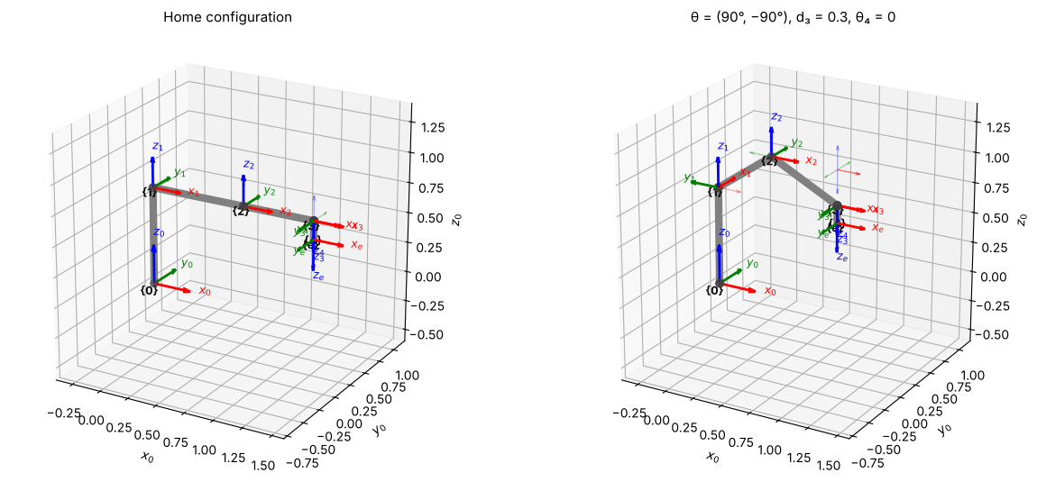
explore(robot_scara, **view_scara)Key Takeaways — Section 5.7
A fixed in flips downward so the quill’s positive direction is “down”.
SCARA: ; the tool always points down with yaw .
5.8 Example 5 — UR5e from a MuJoCo Model¶
The Universal Robots UR5e is a 6-DOF industrial arm. Its geometry here comes from
the MuJoCo Menagerie model universal_robots_ur5e/ur5e.xml, the same kind of MJCF file
you met in Chapter 3. The MJCF uses its own body frames (four of its joint axes are
along a local ), so we re-assign the frames with our Step 1 recipe: along
joint , pointing the same way as the MJCF joint axis, so that equals MuJoCo’s
qpos[i]. Frame is the MuJoCo world frame; at home the arm reaches along .
Parameters (m): , , , , , .
Step 1 — Frames at home ().
| Frame | MJCF joint / site | in frame | |
|---|---|---|---|
| 1 | shoulder_pan_joint | ||
| 2 | shoulder_lift_joint | ||
| 3 | elbow_joint | ||
| 4 | wrist_1_joint | ||
| 5 | wrist_2_joint | ||
| 6 | wrist_3_joint | ||
| e | attachment_site |
Axes 2, 3 and 4 are parallel, and axis 2 meets axis 1, so we may slide along its axis until . The small sideways offsets in the MJCF (0.138, -0.131, 0.127 m) then collapse into the single offset m.
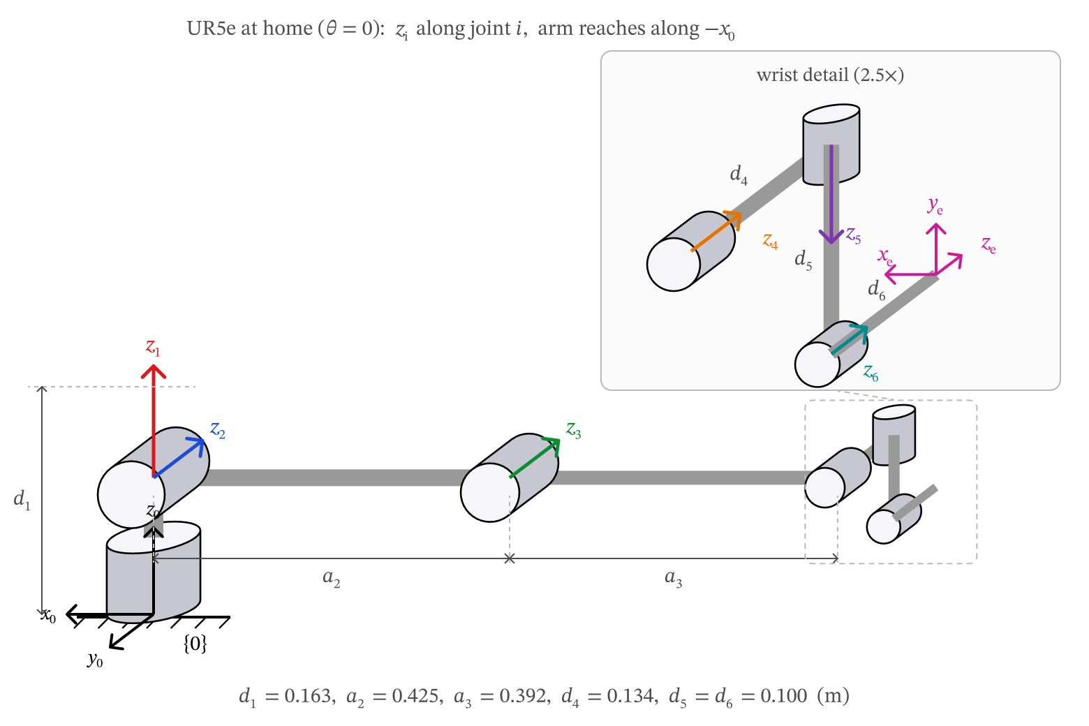
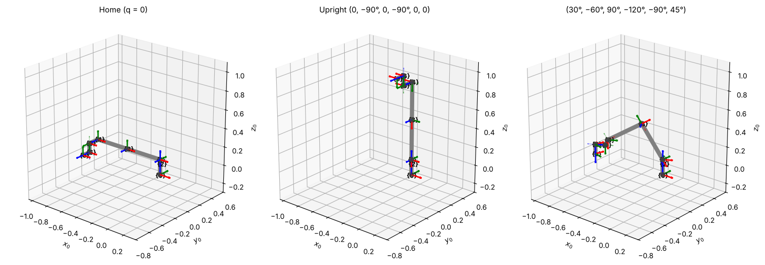
Figure 5.11 — Example 5: UR5e at home with frames re-assigned so zi lies along joint i.
Step 2 — Home configuration and joint motion (all joints revolute):
Step 3 — Multiply. .
This chain was checked against MuJoCo’s own forward kinematics
(data.site_xpos, data.site_xmat of attachment_site) at 500 random joint vectors:
position and orientation agree to about 10-15.
d1, a2, a3, d4, d5, d6 = 0.163, 0.425, 0.392, 0.134, 0.100, 0.100

# Step 2 — home configuration
T_home = [Trans('z', d1),                                 # T_1^0(0)
          Rot('x', np.radians(90)),                       # T_2^1(0)
          Trans('x', -a2),                                # T_3^2(0)
          Trans('x', -a3),                                # T_4^3(0)
          Trans('z', d4) @ Rot('x', np.radians(90)),      # T_5^4(0)
          Trans('z', d5) @ Rot('x', np.radians(-90))]     # T_6^5(0)
Te6 = Trans('z', d6)


def fk_ur5e(q):
    T = np.eye(4)
    for Ti_home, qi in zip(T_home, q):
        T = T @ Ti_home @ Rot('z', qi)      # revolute joint i
    return T @ Te6                          # Step 3


q_up = np.radians([0, -90, 0, -90, 0, 0])
show(fk_ur5e(np.zeros(6)), 'T_e^0 at home (q = 0)')
print()
show(fk_ur5e(q_up), "T_e^0 at the 'upright' pose (0, -90°, 0, -90°, 0, 0)")
T_e^0 at home (q = 0) =
[[ 1. 0. 0. -0.817]
[ 0. 0. -1. -0.234]
[ 0. 1. 0. 0.063]
[ 0. 0. 0. 1. ]]
T_e^0 at the 'upright' pose (0, -90°, 0, -90°, 0, 0) =
[[-1. 0. 0. 0. ]
[ 0. 0. -1. -0.234]
[ 0. -1. 0. 1.08 ]
[ 0. 0. 0. 1. ]]
# Closed-form gripper position (group the terms by link parameter, then simplify)
q = sp.symbols('theta_1:7', real=True)
D1, A2, A3, D4, D5, D6 = sp.symbols('d_1 a_2 a_3 d_4 d_5 d_6', real=True)
sT_home = [sTrans('z', D1), sRot('x', sp.pi/2), sTrans('x', -A2), sTrans('x', -A3),
           sTrans('z', D4) * sRot('x', sp.pi/2), sTrans('z', D5) * sRot('x', -sp.pi/2)]

Te0_ur = sp.eye(4)
for Ti_home, qi in zip(sT_home, q):
    Te0_ur = Te0_ur * Ti_home * sRot('z', qi)
Te0_ur = Te0_ur * sTrans('z', D6)

o_e = sp.Matrix([sp.trigsimp(sp.collect(sp.expand(Te0_ur[i, 3]), [D1, A2, A3, D4, D5, D6]))
                 for i in range(3)])
show_sym(o_e, r'o_e')The closed form is long, but notice the structure: , , only appear through the sums and — the hallmark of three parallel joint axes (compare the terms of the planar 2R arm). does not appear at all: the last joint only rolls the gripper about its own axis. In practice nobody multiplies this out by hand — the three-step procedure plus a computer is the whole point.
robot_ur5e = Robot('Example 5: UR5e (from MJCF)',
                   home=[[Tr('z', d1, 'd_1')],
                         [Rt('x', np.pi/2, r'90^\circ')],
                         [Tr('x', -a2, '-a_2')],
                         [Tr('x', -a3, '-a_3')],
                         [Tr('z', d4, 'd_4'), Rt('x', np.pi/2, r'90^\circ')],
                         [Tr('z', d5, 'd_5'), Rt('x', -np.pi/2, r'-90^\circ')]],
                   joints=[(f'θ{s}', rf'\theta_{i}', 'R', (-180, 180))
                           for i, s in zip(range(1, 7), '₁₂₃₄₅₆')],
                   tool=[Tr('z', d6, 'd_6')])

view_ur5e = dict(center=(-0.35, -0.1, 0.4), half=0.7, view=(22, -50), scale=0.1, axis_labels=False)
q_test = np.radians([30, -60, 90, -120, -90, 45])
print('Robot.fk matches fk_ur5e:', np.allclose(robot_ur5e.fk(q_test), fk_ur5e(q_test)))

snapshot(robot_ur5e, [np.zeros(6), q_up, q_test],
         ['Home (q = 0)', 'Upright (0, −90°, 0, −90°, 0, 0)', '(30°, −60°, 90°, −120°, −90°, 45°)'],
         figsize=(15, 5.5), **view_ur5e)
Robot.fk matches fk_ur5e: True
explore(robot_ur5e, figsize=(7.5, 7), **view_ur5e)Key Takeaways — Section 5.8
The same three steps handle a real 6-DOF industrial arm; the only work is Step 1 (choosing frames) and Step 2 (writing the home transforms).
A robot model file (MJCF, URDF) gives the geometry, but you may re-assign frames to follow our convention — the gripper pose does not change.
Parallel joint axes show up as angle sums (, ) in the closed form.
5.9 The FK Frame Animator and Chapter Summary¶
The FK Frame Animator (Ch5 FK Frame Animator.html, in the same folder as this
notebook) shows all five examples of this chapter as a 3D model you can orbit with the
mouse. It has two modes:
Joint motion: drag the joint sliders (or press Animate joints) and watch every frame ride on its link. The live is shown next to the closed-form position, so you can check your own derivations.
Step through product: the factors of are applied one at a time, each one moving the frame along or about its current axes — the animated version of the
factorsslider used in this notebook.
Run the cell below to open it in your web browser.
from pathlib import Path
import webbrowser

animator = Path('Ch5 FK Frame Animator.html').resolve()
if animator.exists():
    webbrowser.open(animator.as_uri())
    print('Opened', animator)
else:
    print('Put "Ch5 FK Frame Animator.html" in the same folder as this notebook.')
Chapter 5 Summary
An HTM stores the pose of frame relative to ; its columns are , , and expressed in .
Six basic HTMs (, ) build every link transform. A product of them is read left to right, each move about the current axes.
Forward kinematics in three steps:
Frames: on the ground, on link with along joint , at the gripper.
(revolute) or (prismatic).
.
Forward kinematics always has exactly one answer. The reverse problem — find the joint variables that put the gripper at a desired pose — is inverse kinematics, and it is much harder.
| Example | Joints | Gripper position |
|---|---|---|
| Planar 2R | RR | |
| Spherical wrist | RRR | |
| Cylindrical | RPP | |
| SCARA | RRPR | |
| UR5e | RRRRRR | see Section 5.8 |