Chapters 5 to 7 answered where: forward kinematics gives the gripper pose for a set of joint angles, the Jacobian relates their velocities, and inverse kinematics finds the joint angles for a desired gripper pose. A task such as pick and place is therefore a list of poses: above the block, at the block, lifted, above the goal, at the goal. This chapter answers the question in between:
Trajectory generation: given the poses (or joint angles) a robot must pass through, and limits on how fast it may move, find the joint angles as a function of time, , so that the robot moves smoothly, stays within its limits, and finishes quickly.
Two decisions shape every trajectory. The path is the geometric curve the robot follows: a straight line in joint space, a straight line for the gripper, or a curve through several waypoints. The timing is how fast it moves along that path: when it starts, how quickly it speeds up, and when it stops. Good timing makes the motion smooth and keeps the motors within their limits; good path choices keep the gripper away from the table and from objects.
| Section | Topic |
|---|---|
| 8.1 | Paths, trajectories, and time scaling |
| 8.2 | Point-to-point polynomials: linear, cubic, quintic |
| 8.3 | Trapezoidal velocity profiles: the fastest move under speed and acceleration limits |
| 8.4 | Via points: moving through waypoints without stopping |
| 8.5 | Straight-line trajectories in task space |
| 8.6 | From a trajectory to motor commands |
| 8.7 | Putting it together: a fast pick and place on the SO-ARM101 |
Notation (same as Chapters 5 to 7). is the vector of joint
variables; a single joint is . A trajectory runs from at
to at , and is the
distance one joint travels. Dots are time derivatives: is velocity,
acceleration. The formulas work in any units. The one-joint examples use
degrees, because they are easier to read; the robot code works in radians and prints
degrees, as in Chapter 7. In the code, a joint vector is called q.
import numpy as np
import matplotlib.pyplot as plt
from types import SimpleNamespace
from ipywidgets import interact, FloatSlider
%matplotlib inline

np.set_printoptions(precision=4, suppress=True)
Tools and robots from Chapters 5 to 7
The next cell collects what we reuse: the planar 2R arm (, ) with its
forward kinematics, Jacobian and closed-form IK, and the SO-ARM101 with its forward
kinematics (the body frames of its MuJoCo model, Chapter 7) and the analytical position + pitch
IK so101_ik of Section 7.4.3. Run the cell and move on.
# ── Planar 2R arm (Chapters 3, 5 and 6): L1 = 1, L2 = 0.7 ─────────────────────
L1_2R, L2_2R = 1.0, 0.7


def fk_2R(q, L1=L1_2R, L2=L2_2R):
    # Elbow and tip positions of the planar 2R arm; q = (θ1, θ2) in rad (q may be an (N, 2) array)
    q = np.asarray(q, float)
    t1, t12 = q[..., 0], q[..., 0] + q[..., 1]
    elbow = np.stack([L1 * np.cos(t1), L1 * np.sin(t1)], axis=-1)
    tip = elbow + np.stack([L2 * np.cos(t12), L2 * np.sin(t12)], axis=-1)
    return elbow, tip


def jacobian_2R(q, L1=L1_2R, L2=L2_2R):
    # 2x2 Jacobian of the tip position (Chapter 6)
    t1, t12 = q[0], q[0] + q[1]
    return np.array([[-L1 * np.sin(t1) - L2 * np.sin(t12), -L2 * np.sin(t12)],
                     [ L1 * np.cos(t1) + L2 * np.cos(t12),  L2 * np.cos(t12)]])


def ik_2R(x, y, L1=L1_2R, L2=L2_2R, elbow=+1):
    # Closed-form 2R inverse kinematics (Chapter 7, Section 7.1); elbow=+1 gives θ2 > 0
    c2 = (x**2 + y**2 - L1**2 - L2**2) / (2 * L1 * L2)
    th2 = elbow * np.arccos(np.clip(c2, -1, 1))
    th1 = np.arctan2(y, x) - np.arctan2(L2 * np.sin(th2), L1 + L2 * np.cos(th2))
    return np.array([th1, th2])


def draw_2R(ax, q, color='0.4', alpha=1.0, lw=4):
    # Draw the 2R arm as two thick links
    elbow, tip = fk_2R(q)
    pts = np.array([[0, 0], elbow, tip])
    ax.plot(*pts.T, '-', color=color, lw=lw, alpha=alpha, solid_capstyle='round')
    ax.plot(*pts[:2].T, 'o', color=color, ms=5, alpha=alpha)


# ── SO-ARM101: body frames of the MuJoCo model (Chapter 7, Section 7.4) ────────
def Rot(axis, theta):
    c, s = np.cos(theta), np.sin(theta)
    R = {'x': [[1, 0, 0], [0, c, -s], [0, s, c]],
         'y': [[c, 0, s], [0, 1, 0], [-s, 0, c]],
         'z': [[c, -s, 0], [s, c, 0], [0, 0, 1]]}[axis]
    T = np.eye(4)
    T[:3, :3] = R
    return T


def HTM(R, o):
    T = np.eye(4)
    T[:3, :3], T[:3, 3] = R, o
    return T


def quat_to_R(w, x, y, z):
    n = np.sqrt(w*w + x*x + y*y + z*z)
    w, x, y, z = w / n, x / n, y / n, z / n
    return np.array([[1 - 2*(y*y + z*z), 2*(x*y - w*z),     2*(x*z + w*y)],
                     [2*(x*y + w*z),     1 - 2*(x*x + z*z), 2*(y*z - w*x)],
                     [2*(x*z - w*y),     2*(y*z + w*x),     1 - 2*(x*x + y*y)]])


def wrap(angle):
    return (np.asarray(angle) + np.pi) % (2 * np.pi) - np.pi


SO101_LINKS = [
    ('shoulder_pan',  [0.0388353, 0.0, 0.0624],          (0, 0, -1, 0)),
    ('shoulder_lift', [-0.0303992, -0.0182778, -0.0542], (0.5, -0.5, -0.5, -0.5)),
    ('elbow_flex',    [-0.11257, -0.028, 0.0],           (0.707107, 0, 0, 0.707107)),
    ('wrist_flex',    [-0.1349, 0.0052, 0.0],            (0.707107, 0, 0, -0.707107)),
    ('wrist_roll',    [0.0, -0.0611, 0.0181],            (0.0172091, -0.0172091, 0.706897, 0.706897)),
]
SO101_Te5 = HTM(quat_to_R(0.707107, 0, 0.707107, 0), [-0.0079, -0.000218121, -0.0981274])
SO101_LIMITS_DEG = [(-110, 110), (-100, 100), (-96.8, 96.8), (-95, 95), (-157.2, 162.8)]


class SO101:
    def __init__(self):
        self.name, self.n = 'SO-ARM101', 5
        self.joint_names = [name for name, _, _ in SO101_LINKS]
        self.home = [HTM(quat_to_R(*quat), o) for _, o, quat in SO101_LINKS]
        self.lo = np.radians([lo for lo, _ in SO101_LIMITS_DEG])
        self.hi = np.radians([hi for _, hi in SO101_LIMITS_DEG])

    def frames(self, q):
        T, out = np.eye(4), {'0': np.eye(4)}
        for i, (T_home, qi) in enumerate(zip(self.home, q)):
            T = T @ T_home @ Rot('z', qi)
            out[str(i + 1)] = T
        out['e'] = T @ SO101_Te5
        return out

    def fk(self, q):
        return self.frames(q)['e']

    def within_limits(self, q, tol=1e-9):
        return bool(np.all(q >= self.lo - tol) and np.all(q <= self.hi + tol))


so101 = SO101()


def heading(v):
    return np.arctan2(v[1], v[0])


def _arm_plane_geometry():
    F0 = so101.frames(np.zeros(5))
    xp = F0['1'][0, 3]
    S, E, W, P = [np.array([F0[k][0, 3] - xp, F0[k][2, 3]]) for k in ('2', '3', '4', 'e')]
    return SimpleNamespace(xp=xp, S=S, L1=np.linalg.norm(E - S), L2=np.linalg.norm(W - E),
                           L3=np.linalg.norm(P - W), alpha1=heading(E - S),
                           gamma0=np.pi + heading(W - E) - heading(E - S), delta=heading(P - W))


geo = _arm_plane_geometry()


def so101_ik(p_d, phi_d, theta5=0.0, elbow='up'):
    # Analytical position + pitch IK of Chapter 7, Section 7.4.3 (rad). None if out of reach.
    x, y, z = p_d
    theta1 = -np.arctan2(y, x - geo.xp)
    r = np.hypot(x - geo.xp, y)
    W = np.array([r, z]) - geo.L3 * np.array([np.cos(phi_d + geo.delta), np.sin(phi_d + geo.delta)])
    D = np.linalg.norm(W - geo.S)
    c = (geo.L1**2 + geo.L2**2 - D**2) / (2 * geo.L1 * geo.L2)
    if abs(c) > 1:
        return None
    gamma = np.arccos(c)
    sigma = np.arccos(np.clip((geo.L1**2 + D**2 - geo.L2**2) / (2 * geo.L1 * D), -1, 1))
    psi_sw = heading(W - geo.S)
    if elbow == 'up':
        theta3, theta2 = geo.gamma0 - gamma, geo.alpha1 - (psi_sw + sigma)
    else:
        theta3, theta2 = geo.gamma0 + gamma - 2 * np.pi, geo.alpha1 - (psi_sw - sigma)
    theta4 = -phi_d - theta2 - theta3
    return wrap(np.array([theta1, theta2, theta3, theta4, theta5]))


print('Ready: planar 2R arm (fk_2R, jacobian_2R, ik_2R) and SO-ARM101 (so101.fk, so101_ik).')
Ready: planar 2R arm (fk_2R, jacobian_2R, ik_2R) and SO-ARM101 (so101.fk, so101_ik).
8.1 Paths, Trajectories, and Time Scaling
A path is a curve through the space of joint angles, written with a path parameter that runs from 0 at the start to 1 at the end: , . The simplest path is the straight line in joint space,
A trajectory adds timing: a time scaling says how far along the path the robot is at time , with and . The trajectory is , and by the chain rule
On the straight line, and , so every joint moves in proportion to the distance it has to travel. Writing for the distance joint travels (the -th entry of ),
All joints start together, stop together, and reach their peak speed at the same instant. Separating the path from the timing lets us design once (Sections 8.2 and 8.3) and use it for any path: a line in joint space here, a line for the gripper in Section 8.5.
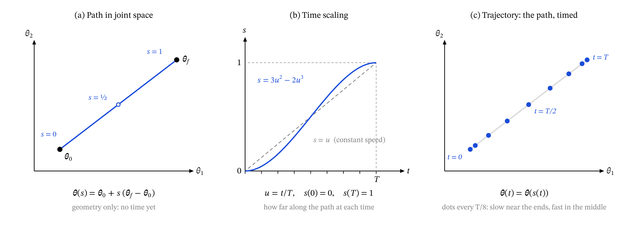
Figure 8.1 — Path + timing = trajectory. (a) A straight path in joint space, parameterized by s. (b) A time scaling s(t): the cubic of Section 8.2 (blue) and constant speed (dashed). (c) The path sampled at equal times: close together at the ends, far apart in the middle.
Figure 8.1 puts the two pieces together.
The scaling law. Write the time scaling with the normalized time , as . Then and , where is :
Stretching a trajectory in time by a factor divides its velocities by and its accelerations by . To bring a trajectory within a velocity limit and an acceleration limit , stretch it by .
What makes a good time scaling? At rest before and after the move, so at both ends. Velocity must be continuous: a jump in velocity needs an infinite acceleration, and the torque a motor must supply grows with acceleration, so a real joint cannot follow a jump and lags behind. Ideally the acceleration is continuous too, because a sudden step in torque shakes the arm. And it should be as fast as the motors allow. Sections 8.2 and 8.3 trade these goals against each other.
The plot below shows the 2R arm on the same straight joint-space path with two time scalings, drawn at nine equally spaced times. The path is identical; only the spacing changes.
q_a, q_b = np.radians([-30, 100]), np.radians([60, 20])
scalings = [('constant speed:  s = u', lambda u: u),
            ('smooth start and stop:  s = 3u² − 2u³ (Section 8.2)', lambda u: 3 * u**2 - 2 * u**3)]

fig, axes = plt.subplots(1, 2, figsize=(13, 5))
for ax, (title, s_of_u) in zip(axes, scalings):
    u_fine = np.linspace(0, 1, 200)
    tip_path = fk_2R(q_a + np.outer(s_of_u(u_fine), q_b - q_a))[1]
    ax.plot(*tip_path.T, color='0.6', lw=1.5, ls='--', label='tip path')
    for k, u in enumerate(np.linspace(0, 1, 9)):
        q = q_a + s_of_u(u) * (q_b - q_a)
        draw_2R(ax, q, color=plt.cm.viridis(k / 8), alpha=0.8, lw=3)
        ax.plot(*fk_2R(q)[1], 'o', color=plt.cm.viridis(k / 8), ms=7)
    ax.set_title(title, fontsize=11)
    ax.set_aspect('equal'); ax.grid(alpha=0.3); ax.set_xlim(-0.5, 1.8); ax.set_ylim(-0.9, 1.6)
    ax.legend(loc='lower left')
fig.suptitle('Same path, two time scalings: the arm at t = 0, T/8, ..., T (dark to light)', fontsize=12)
plt.tight_layout(); plt.show()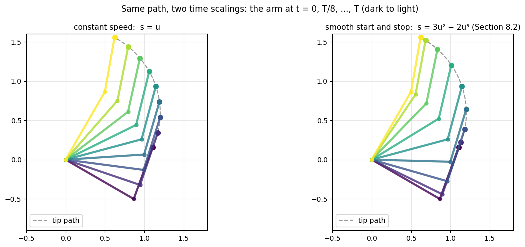
With constant speed the tip advances equal distances in equal times, from the first instant to the last. The smooth scaling starts gently, covers most of the path in the middle of the move, and slows down into the goal.
Key Takeaways — Section 8.1
Path = geometry, ; trajectory = path + timing, .
On a straight joint-space path, and : all joints share one time scaling and finish together.
Scaling law: stretching the time by divides velocities by and accelerations by .
Goals: start and end at rest, continuous velocity (ideally continuous acceleration), within the limits, fast.
8.2 Point-to-Point Polynomials
8.2.1 Linear interpolation
The simplest time scaling is constant speed, :
where is the distance the joint travels. (From here on, the formulas are for one joint, so we drop the index ; for the whole arm, apply them to each joint with its own .)
It is what a program does when it simply sends evenly spaced goal positions to a servo. Its velocity jumps from 0 to at and back to 0 at , so the acceleration is infinite at those two instants. The motor cannot follow: a position servo falls behind as soon as a linear move starts, trails behind the command for the whole move, and arrives late and still moving (Section 8.6 models this). Linear interpolation is fine for slow, small moves; for anything quick we need a velocity that starts and ends at zero.
8.2.2 Cubic polynomials
Take one joint. We want it to start at with velocity and to reach with velocity at time . Four conditions need four free coefficients, so we use a cubic:
The four conditions are four linear equations in the coefficients:
The first two rows give and . Substituting them into the last two rows leaves two equations in and , with the solution
Rest to rest (): , , , . To see the time scaling inside this cubic, substitute the coefficients and factor out :
With the normalized time (from 0 at the start to 1 at the end), the bracket depends on alone. Comparing with the straight path of Section 8.1, , the bracket is the time scaling:
where is . It satisfies , and , and it is the same for every joint and every move; only and change. To get back to time, use the chain rule with (Section 8.1):
The velocity is a parabola, zero at both ends, with its peak at the middle: , 50% faster than linear interpolation, because the cubic makes up for its slow start and finish. The acceleration falls linearly from to : finite everywhere, but it still jumps from 0 to at the start and back to 0 at the end. The velocity is continuous; the acceleration is not.
We keep and in the formulas because Section 8.4 strings cubics together through waypoints without stopping, which needs nonzero velocities at the joins. The cell codes the formulas and checks them against solving numerically.
def cubic_coefficients(q0, qf, T, v0=0.0, vf=0.0):
    # Coefficients [a0, a1, a2, a3] of the cubic with q(0) = q0, q'(0) = v0, q(T) = qf, q'(T) = vf
    a2 = (3 * (qf - q0) - (2 * v0 + vf) * T) / T**2
    a3 = (-2 * (qf - q0) + (v0 + vf) * T) / T**3
    return np.array([q0, v0, a2, a3])


def poly_eval(a, t):
    # Position, velocity and acceleration of the polynomial a[0] + a[1] t + a[2] t^2 + ... (t may be an array)
    t = np.asarray(t, float)
    q   = sum(a[k] * t**k for k in range(len(a)))
    qd  = sum(k * a[k] * t**(k - 1) for k in range(1, len(a)))
    qdd = sum(k * (k - 1) * a[k] * t**(k - 2) for k in range(2, len(a)))
    return q, qd, qdd


q0, qf, T, v0, vf = -30.0, 45.0, 2.0, 10.0, -5.0                   # degrees, seconds
M = np.array([[1, 0, 0, 0], [0, 1, 0, 0], [1, T, T**2, T**3], [0, 1, 2 * T, 3 * T**2]])
print('formulas        :', cubic_coefficients(q0, qf, T, v0, vf))
print('np.linalg.solve :', np.linalg.solve(M, [q0, v0, qf, vf]))

a = cubic_coefficients(0.0, 90.0, 2.0)                             # rest to rest: 90° in 2 s
q, qd, qdd = poly_eval(a, np.linspace(0, 2.0, 2001))
print(f'\nRest to rest, Δ = 90°, T = 2 s: peak velocity {qd.max():.2f}°/s (1.5 Δ/T = {1.5 * 90 / 2:.2f}), '
      f'acceleration at the ends ±{qdd.max():.1f}°/s² (6 Δ/T² = {6 * 90 / 4:.1f})')
formulas : [-30. 10. 48.75 -17.5 ]
np.linalg.solve : [-30. 10. 48.75 -17.5 ]
Rest to rest, Δ = 90°, T = 2 s: peak velocity 67.50°/s (1.5 Δ/T = 67.50), acceleration at the ends ±135.0°/s² (6 Δ/T² = 135.0)
Explore the end velocities. The sliders set , and for a 90° move. With small end velocities the cubic is an S-curve. Make large and the joint overshoots and comes back; make it negative and the joint first moves the wrong way. Large end velocities in a short time are exactly what makes multi-segment trajectories wander (Section 8.4).
def explore_cubic():
    def _view(v0=0.0, vf=0.0, T=2.0):
        a = cubic_coefficients(0.0, 90.0, T, v0, vf)
        t = np.linspace(0, T, 400)
        q, qd, qdd = poly_eval(a, t)
        fig, axes = plt.subplots(1, 3, figsize=(15, 3.6))
        for ax, y, label in zip(axes, (q, qd, qdd), ('position (°)', 'velocity (°/s)', 'acceleration (°/s²)')):
            ax.plot(t, y, lw=2)
            ax.set_xlabel('t (s)'); ax.set_ylabel(label); ax.grid(alpha=0.3)
        axes[0].axhline(90, color='k', ls=':', lw=1)
        axes[0].set_title(f'cubic from 0° to 90°: max {q.max():.1f}°, min {q.min():.1f}°')
        plt.tight_layout(); plt.show()

    interact(_view,
             v0=FloatSlider(value=0, min=-150, max=150, step=5, description='v₀ (°/s)'),
             vf=FloatSlider(value=0, min=-150, max=150, step=5, description='v_f (°/s)'),
             T=FloatSlider(value=2.0, min=0.5, max=4.0, step=0.1, description='T (s)'))


explore_cubic()8.2.3 Quintic polynomials
To remove the jump in acceleration we also fix the accelerations at both ends, which makes six conditions, so we need a quintic (degree 5):
with , , , and , , . As before, the conditions at give the first coefficients directly (, , ), and the three conditions at form a linear system for . For rest to rest with zero end accelerations the solution is
Now the velocity and the acceleration start and end at zero. The price is a higher peak speed, , at the middle of the move. The peak acceleration is , a little lower than the cubic’s, and it occurs at instead of at the ends.
The pattern continues: the derivative of acceleration, the jerk, now jumps at the ends, and a degree-7 polynomial with eight conditions makes the jerk start and end at zero too. Each step makes the start gentler and the middle faster.
The general solution is easiest to compute numerically from the system:
def quintic_coefficients(q0, qf, T, v0=0.0, vf=0.0, acc0=0.0, accf=0.0):
    # Coefficients [a0, ..., a5] of the quintic with given position, velocity and acceleration at both ends
    M = np.array([[1, 0, 0,     0,        0,         0],
                  [0, 1, 0,     0,        0,         0],
                  [0, 0, 2,     0,        0,         0],
                  [1, T, T**2,  T**3,     T**4,      T**5],
                  [0, 1, 2 * T, 3 * T**2, 4 * T**3,  5 * T**4],
                  [0, 0, 2,     6 * T,    12 * T**2, 20 * T**3]])
    return np.linalg.solve(M, [q0, v0, acc0, qf, vf, accf])


T, D = 2.0, 90.0
print('quintic, rest to rest :', np.round(quintic_coefficients(0.0, D, T), 6))
print('closed form           :', np.round([0, 0, 0, 10 * D / T**3, -15 * D / T**4, 6 * D / T**5], 6))
quintic, rest to rest : [ 0. 0. 0. 112.5 -84.375 16.875]
closed form : [ 0. 0. 0. 112.5 -84.375 16.875]
8.2.4 Comparing the profiles, and choosing 
The plot shows the three rest-to-rest time scalings in normalized form: , and against . Multiply the velocity axis by and the acceleration axis by to get a joint’s actual values.
u = np.linspace(-0.15, 1.15, 1301)
uc = np.clip(u, 0, 1)
moving = (u > 0) & (u < 1)
profiles = {
    'linear':  (uc,                             np.where(moving, 1.0, 0.0),           np.zeros_like(u)),
    'cubic':   (3 * uc**2 - 2 * uc**3,          np.where(moving, 6 * uc * (1 - uc), 0), np.where(moving, 6 - 12 * uc, 0)),
    'quintic': (10 * uc**3 - 15 * uc**4 + 6 * uc**5,
                np.where(moving, 30 * uc**2 * (1 - uc)**2, 0),
                np.where(moving, 60 * uc - 180 * uc**2 + 120 * uc**3, 0)),
}

fig, axes = plt.subplots(1, 3, figsize=(16, 4))
for name, (s, sd, sdd) in profiles.items():
    for ax, y in zip(axes, (s, sd, sdd)):
        ax.plot(u, y, lw=2, label=name)
for ax, label in zip(axes, ("s", "s'  (× Δ/T for velocity)", "s''  (× Δ/T² for acceleration)")):
    ax.set_xlabel('u = t/T'); ax.set_ylabel(label); ax.grid(alpha=0.3); ax.legend()
axes[2].text(0.30, 0.06, 'linear: infinite at u = 0 and u = 1', transform=axes[2].transAxes, color='tab:blue')
plt.tight_layout(); plt.show()

print(f"{'profile':<9} {'peak velocity':>15} {'peak acceleration':>19}   continuous up to")
for name, cont in [('linear', 'position'), ('cubic', 'velocity'), ('quintic', 'acceleration')]:
    s, sd, sdd = profiles[name]
    acc = 'infinite' if name == 'linear' else f'{np.abs(sdd).max():.3f} Δ/T²'
    print(f'{name:<9} {sd.max():10.3f} Δ/T {acc:>19}   {cont}')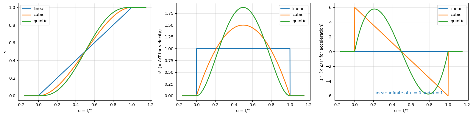
profile     peak velocity   peak acceleration   continuous up to
linear         1.000 Δ/T            infinite   position
cubic          1.500 Δ/T          6.000 Δ/T²   velocity
quintic        1.875 Δ/T          5.773 Δ/T²   acceleration
Choosing from the motor limits. Suppose a joint may move at most and accelerate at most . A rest-to-rest polynomial with peak values and stays within both limits if
Several joints. All joints share one time scaling (Section 8.1), so the joint that needs the most time sets for everyone; the others move more slowly than their limits allow, and all arrive together.
Example limits. For the SO-ARM101 we use and for every arm joint throughout this chapter. These are illustrative values. The real limits depend on the servos, the supply voltage, the load, and how firmly the gripper holds the block, and are best measured on the robot: the pan joint of one 12 V SO-ARM101, for example, reached about 200°/s and 2,000°/s². The example move goes from 6 cm above a pick spot at cm to 6 cm above a place spot at cm, with the gripper pointing straight down.
V_MAX = np.radians(180.0)            # rad/s   example joint speed limit (every arm joint)
A_MAX = np.radians(720.0)            # rad/s²  example joint acceleration limit
PHI_DOWN = np.radians(-90.0)         # gripper pointing straight down
Z_GRASP, LIFT = 0.015, 0.06          # gripper-point height for grasping a 1-inch block, and lift height (m)
PICK_XY, PLACE_XY = np.array([0.20, -0.12]), np.array([0.20, 0.0])   # pick and place spots (x, y) (m)


def so101_top_down(xy, z):
    # Joint vector (rad) that puts the gripper point at (x, y, z), pointing straight down
    q = so101_ik(np.array([*xy, z]), PHI_DOWN)
    assert q is not None and so101.within_limits(q), f'{xy}, z = {z}: not reachable top-down'
    return q


def poly_min_time(delta, v_max, a_max, cv, ca):
    # Shortest T for a rest-to-rest polynomial with peak velocity cv Δ/T and peak acceleration ca Δ/T²
    return max(cv * np.abs(delta) / v_max, np.sqrt(ca * np.abs(delta) / a_max))


q_start, q_goal = so101_top_down(PICK_XY, Z_GRASP + LIFT), so101_top_down(PLACE_XY, Z_GRASP + LIFT)
delta = q_goal - q_start
print(f"{'joint':<15}{'Δ (°)':>8}{'T_min cubic (s)':>18}{'T_min quintic (s)':>20}")
for name, d in zip(so101.joint_names, delta):
    print(f'{name:<15}{np.degrees(d):8.1f}{poly_min_time(d, V_MAX, A_MAX, 1.5, 6):18.3f}'
          f'{poly_min_time(d, V_MAX, A_MAX, 1.875, 10 / np.sqrt(3)):20.3f}')
T_cubic = max(poly_min_time(d, V_MAX, A_MAX, 1.5, 6) for d in delta)
print(f'\nAll joints together with one cubic: T = {T_cubic:.3f} s, set by shoulder_pan')
joint Δ (°) T_min cubic (s) T_min quintic (s)
shoulder_pan -36.7 0.553 0.542
shoulder_lift -20.4 0.412 0.404
elbow_flex 24.0 0.447 0.439
wrist_flex -3.6 0.174 0.171
wrist_roll 0.0 0.000 0.000
All joints together with one cubic: T = 0.553 s, set by shoulder_pan
shoulder_pan has the farthest to go, so it sets ; the other joints move only a few
degrees and use a small part of their limits. Its comes from the acceleration
limit, not the speed limit: for moves shorter than (120° for
the cubic with these limits) the square root wins.
Key Takeaways — Section 8.2
Linear interpolation: constant speed , but velocity jumps at both ends (infinite acceleration).
Cubic: four conditions ; , . Rest to rest: , peak velocity , acceleration at the ends (it jumps there).
Quintic: six conditions, adds the end accelerations; rest to rest , peak velocity , acceleration continuous.
Choose from the limits: ; with several joints the slowest joint sets .
8.3 Trapezoidal Velocity Profiles
8.3.1 Accelerate, cruise, decelerate
The polynomials of Section 8.2 never use their full speed or acceleration for long: the cubic reaches its peak speed only for an instant, and its acceleration falls steadily. A trapezoidal velocity profile uses both limits as much as possible. It has three phases:
accelerate at constant for a time , until the speed reaches ;
cruise at constant speed ;
decelerate at for , coming to rest at .
The velocity is a trapezoid and the position is a parabola, a straight line, and a parabola, so the profile is also called linear segment with parabolic blends (LSPB). The area under the velocity is the distance travelled, , so
During the move (for ):
The cruise phase exists only if , that is . A move too short to reach becomes a triangle: accelerate for half the time, decelerate for the other half, peak speed and .
Sometimes is given instead (for example, to make one joint finish together with another). Fix the acceleration and solve for the blend time:
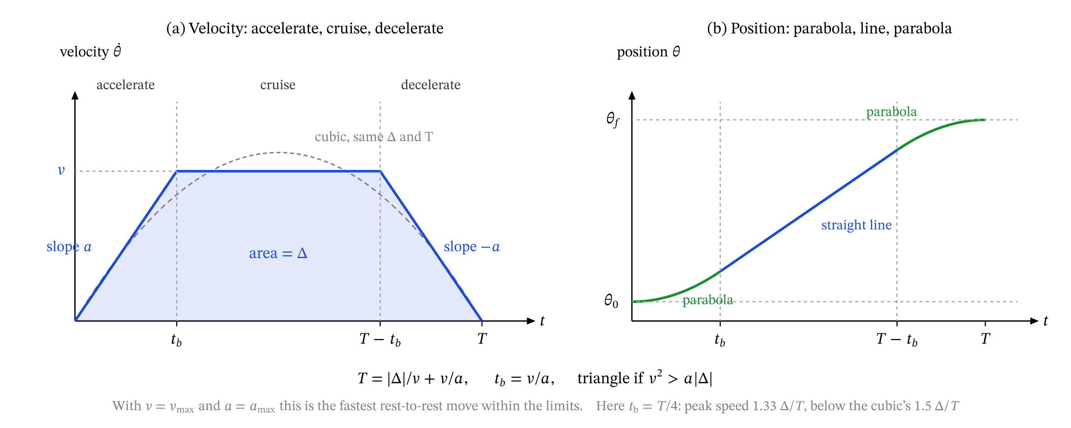
Figure 8.2 — Anatomy of a trapezoidal velocity profile. (a) Velocity: accelerate at a for tb, cruise at v, decelerate; the area under the curve is the distance Δ. The dashed curve is a cubic with the same Δ and T. (b) Position: parabola, straight line, parabola.
def trapezoid_min_time(delta, v_max, a_max):
    # Fastest rest-to-rest move of size |delta| with |speed| <= v_max and |acceleration| <= a_max.
    # Returns (T, v, t_b): total time, cruise speed reached, and acceleration (blend) time.
    d = abs(delta)
    v = v_max if d * a_max >= v_max**2 else np.sqrt(d * a_max)    # trapezoid, or triangle if too short
    t_b = v / a_max
    return d / v + t_b, v, t_b


def trapezoid_eval(q0, qf, T, t_b, t):
    # Position, velocity and acceleration at time t (scalar or array) of the trapezoid from q0 to qf
    t = np.clip(np.asarray(t, float), 0, T)
    v = (qf - q0) / (T - t_b)                                      # signed cruise velocity
    a = v / t_b
    accel, decel = t < t_b, t > T - t_b
    q = np.where(accel, q0 + 0.5 * a * t**2, np.where(decel, qf - 0.5 * a * (T - t)**2, q0 + v * (t - t_b / 2)))
    qd = np.where(accel, a * t, np.where(decel, a * (T - t), v))
    qdd = np.where(accel, a, np.where(decel, -a, 0.0))
    return q, qd, qdd


def trapezoid_blend_time(delta, T, a):
    # Blend time of the trapezoid that moves |delta| in exactly T with acceleration a (needs a T² >= 4|delta|)
    disc = T**2 - 4 * abs(delta) / a
    assert disc >= 0, 'T too short for this acceleration'
    return (T - np.sqrt(disc)) / 2


T, v, t_b = trapezoid_min_time(90.0, 180.0, 720.0)              # 90° with 180°/s and 720°/s²
t = np.linspace(0, T, 1001)
q, qd, qdd = trapezoid_eval(0.0, 90.0, T, t_b, t)
fig, axes = plt.subplots(1, 3, figsize=(15, 3.8))
for ax, y, label in zip(axes, (q, qd, qdd), ('position (°)', 'velocity (°/s)', 'acceleration (°/s²)')):
    ax.plot(t, y, lw=2)
    for tb_line in (t_b, T - t_b):
        ax.axvline(tb_line, color='0.6', ls=':')
    ax.set_xlabel('t (s)'); ax.set_ylabel(label); ax.grid(alpha=0.3)
axes[1].text(t_b / 2, v * 0.5, 'accelerate', ha='center'); axes[1].text(T / 2, v * 0.9, 'cruise', ha='center')
axes[1].text(T - t_b / 2, v * 0.5, 'decelerate', ha='center')
plt.tight_layout(); plt.show()
print(f'Δ = 90°: T = {T:.3f} s, cruise at {v:.0f}°/s, blend time t_b = {t_b:.3f} s; '
      f'check: end position {q[-1]:.4f}°')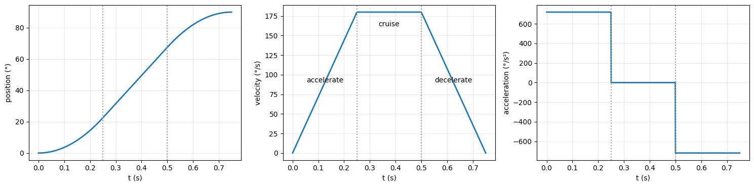
Δ = 90°: T = 0.750 s, cruise at 180°/s, blend time t_b = 0.250 s; check: end position 90.0000°
8.3.2 The fastest move under speed and acceleration limits
With and the trapezoid is the fastest possible rest-to-rest move within the two limits. The reason: to cover as quickly as possible the joint must be as fast as possible at every instant. It cannot speed up faster than , cannot cruise faster than , and must still be able to stop in time, which it does only by braking at at the last possible moment. The trapezoid does exactly that. This “full acceleration, full speed, full braking” structure is called bang-coast-bang.
The cell compares the shortest time of each profile for several move sizes, with the example limits of Section 8.2.4.
v_lim, a_lim = 180.0, 720.0                                      # °/s, °/s²
print(f'Shortest rest-to-rest time (s) with v_max = {v_lim:.0f}°/s, a_max = {a_lim:.0f}°/s²\n')
print(f"{'Δ (°)':>6} {'trapezoid':>10} {'cubic':>8} {'quintic':>8}   trapezoid saves")
for D in (10, 20, 45, 90, 180):
    T_trap = trapezoid_min_time(D, v_lim, a_lim)[0]
    T_cub = poly_min_time(D, v_lim, a_lim, 1.5, 6)
    T_qui = poly_min_time(D, v_lim, a_lim, 1.875, 10 / np.sqrt(3))
    print(f'{D:6d} {T_trap:10.3f} {T_cub:8.3f} {T_qui:8.3f}   {100 * (1 - T_trap / T_cub):5.1f}% vs cubic')

D = 90.0
fig, axes = plt.subplots(1, 2, figsize=(14, 4))
T_trap, _, t_b = trapezoid_min_time(D, v_lim, a_lim)
t = np.linspace(0, T_trap, 500)
_, qd, qdd = trapezoid_eval(0, D, T_trap, t_b, t)
axes[0].plot(t, qd, lw=2, label=f'trapezoid, T = {T_trap:.3f} s'); axes[1].plot(t, qdd, lw=2)
for name, cv, ca in [('cubic', 1.5, 6), ('quintic', 1.875, 10 / np.sqrt(3))]:
    Tp = poly_min_time(D, v_lim, a_lim, cv, ca)
    coeffs = cubic_coefficients(0, D, Tp) if name == 'cubic' else quintic_coefficients(0, D, Tp)
    t = np.linspace(0, Tp, 500)
    _, qd, qdd = poly_eval(coeffs, t)
    axes[0].plot(t, qd, lw=2, label=f'{name}, T = {Tp:.3f} s'); axes[1].plot(t, qdd, lw=2)
for ax, lim, label in [(axes[0], v_lim, 'velocity (°/s)'), (axes[1], a_lim, 'acceleration (°/s²)')]:
    ax.axhline(lim, color='crimson', ls='--', lw=1); ax.axhline(-lim, color='crimson', ls='--', lw=1)
    ax.set_xlabel('t (s)'); ax.set_ylabel(label); ax.grid(alpha=0.3)
axes[0].legend(); axes[0].set_title(f'Δ = {D:.0f}°, each at its shortest time (dashed: limits)')
plt.tight_layout(); plt.show()
Shortest rest-to-rest time (s) with v_max = 180°/s, a_max = 720°/s²
Δ (°) trapezoid cubic quintic trapezoid saves
10 0.236 0.289 0.283 18.4% vs cubic
20 0.333 0.408 0.400 18.4% vs cubic
45 0.500 0.612 0.601 18.4% vs cubic
90 0.750 0.866 0.938 13.4% vs cubic
180 1.250 1.500 1.875 16.7% vs cubic
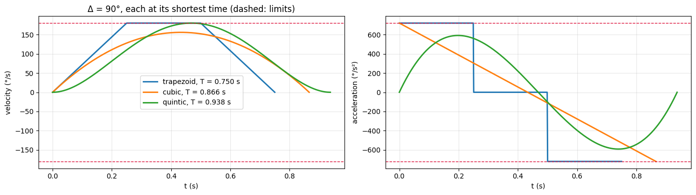
The trapezoid is 13% to 18% faster than the cubic over this range, and more than that against the quintic for long moves: it rides along both limits, while the polynomials touch each limit only at one instant.
Smoothness. The trapezoid’s acceleration jumps four times (at the start and end of each blend), so like the cubic it has continuous velocity but not continuous acceleration. Industrial drives often use an S-curve profile, which also limits the jerk by ramping the acceleration up and down linearly; it is a trapezoid of acceleration inside a smooth velocity profile.
Servos do this too. Sent a single goal angle, a smart servo such as the STS3215 of the SO-ARM101 runs its own trapezoidal velocity profile toward the goal. Section 8.6 discusses how that built-in profile interacts with the trajectories of this chapter.
8.3.3 Synchronizing several joints
If each joint ran its own fastest trapezoid, the joints would finish at different times and the arm would not follow the straight joint-space path. Instead, give all joints one trapezoidal time scaling . Since and , every joint stays within its limits if
and the fastest such is the trapezoid from 0 to 1 with limits and . The joint with the largest (relative to its limits) uses its full speed and acceleration; the others scale down in proportion.
def sync_trapezoid(q0, qf, v_max, a_max):
    # One trapezoidal time scaling for all joints, as fast as the limits allow.
    # v_max, a_max: scalars or one value per joint. Returns (T, traj) with traj(t) -> (q, qd, qdd).
    q0, qf = np.asarray(q0, float), np.asarray(qf, float)
    d = np.abs(qf - q0)
    moving = d > 1e-12
    sd_max = np.min(np.broadcast_to(v_max, d.shape)[moving] / d[moving])
    sdd_max = np.min(np.broadcast_to(a_max, d.shape)[moving] / d[moving])
    T, _, t_b = trapezoid_min_time(1.0, sd_max, sdd_max)

    def traj(t):
        s, sd, sdd = trapezoid_eval(0.0, 1.0, T, t_b, t)
        return q0 + s * (qf - q0), sd * (qf - q0), sdd * (qf - q0)
    return T, traj


def sample(traj, T, n=601):
    # Sample traj(t) -> (q, qd, qdd) at n times from 0 to T; returns t and three (n, dof) arrays
    t = np.linspace(0, T, n)
    q, qd, qdd = (np.array(x) for x in zip(*(traj(ti) for ti in t)))
    return t, q, qd, qdd


T_sync, traj_sync = sync_trapezoid(q_start, q_goal, V_MAX, A_MAX)
t, q, qd, qdd = sample(traj_sync, T_sync)

fig, axes = plt.subplots(1, 2, figsize=(14, 4), sharey=True)
for i, name in enumerate(so101.joint_names[:4]):
    Ti, _, tbi = trapezoid_min_time(delta[i], V_MAX, A_MAX)
    ti = np.linspace(0, Ti, 300)
    axes[0].plot(ti, np.degrees(trapezoid_eval(q_start[i], q_goal[i], Ti, tbi, ti)[1]), lw=2, label=f'{name} ({Ti:.2f} s)')
    axes[1].plot(t, np.degrees(qd[:, i]), lw=2, label=name)
axes[0].set_title('Each joint on its own fastest trapezoid'); axes[1].set_title(f'One shared time scaling: all finish at T = {T_sync:.3f} s')
for ax in axes:
    ax.set_xlabel('t (s)'); ax.grid(alpha=0.3); ax.legend(fontsize=9)
axes[0].set_ylabel('joint velocity (°/s)')
plt.tight_layout(); plt.show()
print(f'Synchronized trapezoid: T = {T_sync:.3f} s   (one cubic within the same limits: {T_cubic:.3f} s)')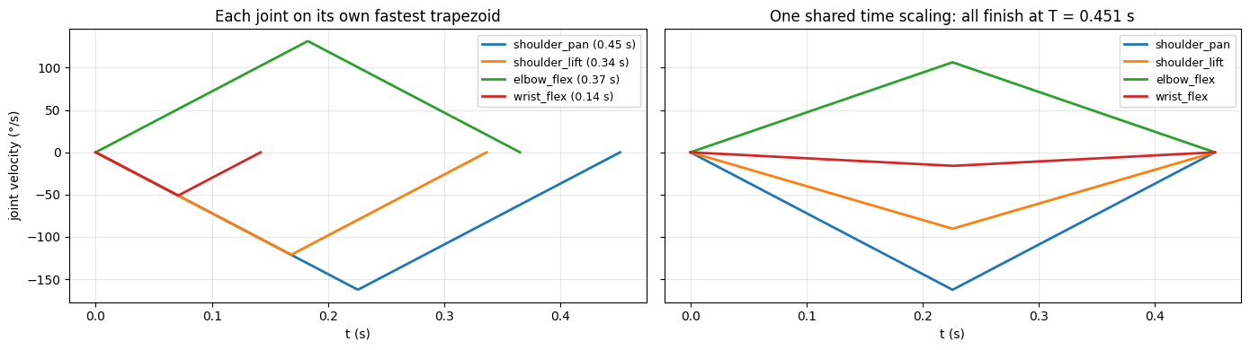
Synchronized trapezoid: T = 0.451 s (one cubic within the same limits: 0.553 s)
On the left, the joints finish at different times, so the arm leaves the straight joint-space path between the two poses; the gripper’s pitch, , changes during the move because the three joints no longer move in step. On the right, every joint follows the same profile shape, scaled by its distance, and they all arrive together, in the time the pan joint needs anyway.
| Profile | Peak velocity | Peak acceleration | Continuous up to | Use | |
|---|---|---|---|---|---|
| Linear | infinite (ends) | position | slow moves only | ||
| Cubic | (ends) | velocity | simple and smooth; also passes through points with given velocities (Section 8.4) | ||
| Quintic | acceleration | gentlest start and stop | |||
| Trapezoid | accelerate, cruise, decelerate | (e.g. ) | (e.g. ) | velocity | fastest within , |
Key Takeaways — Section 8.3
Trapezoid (LSPB): accelerate at for , cruise at , decelerate; ; a triangle if .
With and it is the fastest rest-to-rest move within the limits (bang-coast-bang), about 15% faster than the cubic.
For a given : .
Synchronize joints with one time scaling: , .
8.4 Via Points: Moving Through Waypoints Without Stopping
A pick and place visits a sequence of waypoints: above the block, down to the block (close the gripper), back up, over to above the goal, down (open the gripper), and up again. With a rest-to-rest move between each pair, the arm stops at every waypoint, and every stop costs time: the arm must slow down to zero and speed up again.
Only some waypoints need a stop. At the block and at the goal the arm must be at rest while the gripper closes or opens. The points above them are there to shape the path, so that the block is lifted clear of the table and lowered from above; the arm only needs to pass through or near them. These are via points. This section gives two ways to pass via points without stopping:
Cubic segments with nonzero velocities at the via points (Section 8.4.1): the trajectory passes exactly through every point.
Linear segments with parabolic blends (Section 8.4.2): the trapezoid of Section 8.3, extended to many points; the trajectory passes near the via points and rounds the corners.
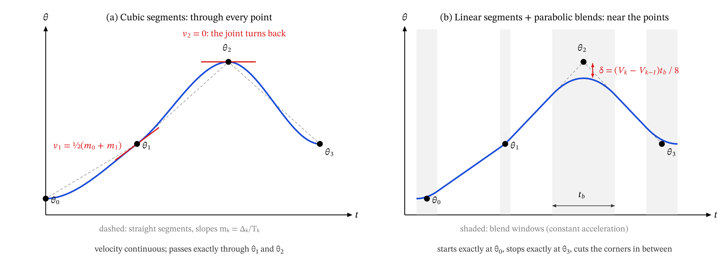
Figure 8.3 — Two ways through via points. (a) Cubic segments with a velocity vk at each via point pass exactly through every point; a joint that turns back gets v = 0. (b) Linear segments with parabolic blends (shaded) start and stop exactly at the end points but miss each via point by δ = (Vk − Vk−1) tb/8.
8.4.1 Cubic segments with velocities at the via points
Let the waypoints be for one joint: the start, via points, and the goal. Segment () runs from to in time , with , and each segment is a cubic of Section 8.2.2.
Count the unknowns and the conditions. cubic segments have coefficients. The conditions we certainly want are:
| Condition | Equations |
|---|---|
| each segment starts at and ends at | |
| the joint starts and ends at rest | 2 |
| the velocity is continuous at each via point | |
| total |
That leaves conditions to choose: one per via point. A convenient way to see them is to name the velocity at each waypoint, , and build segment as the cubic from to with the formulas of Section 8.2.2. Then the first conditions hold automatically: each segment hits its two waypoints, gives the rest conditions, and neighbouring segments share , so the velocity is continuous. The only unknowns left are the via velocities , and we need equations for them. The two rules below supply those equations in different ways.
Rule 1: average the slopes (one explicit formula per via point). Let be the average speed of segment . At via point ,
This gives the equations directly, each via velocity on its own, so nothing has to be solved. A joint that keeps moving the same way passes through at about its average speed; a joint that turns back stops at its turning point. Nothing in it asks for continuous acceleration, so the acceleration jumps at the via points.
Rule 2: continuous acceleration (the cubic spline). Use the free conditions to make the acceleration continuous at every via point. From the coefficients of Section 8.2.2, a cubic segment with end velocities has the accelerations
at its two ends. (They follow from : and , with , from Section 8.2.2.)
At via point , two segments meet. The segment arriving is segment : it has and , starts with and ends with . The segment leaving is segment : it has and , starts with and ends with . Their accelerations at the via point are
Set them equal and split each fraction:
Move the velocities to the left and the terms to the right:
Divide by 2 and group the two terms. This gives one equation at each via point :
That is linear equations for the unknowns ( are known), so the count closes: conditions for coefficients, and the solution is unique. Unlike Rule 1, the via velocities are coupled: each equation involves a via velocity and its two neighbours, so they must be solved together. The matrix is tridiagonal. For the five waypoints used below ( segments, 16 coefficients, 3 via points):
(the terms with and drop out because both are zero). The solution is the cubic spline through the waypoints. Among all trajectories that pass through the waypoints at the given times and start and end at rest, the spline has the smallest : in that sense it is the smoothest.
| Unknowns | Equations | How they are found | |
|---|---|---|---|
| Stop at every point | none | — | |
| Rule 1: average slopes | via velocities | , one per via point | each computed on its own |
| Rule 2: cubic spline | via velocities | , one per via point | one tridiagonal linear system |
The cell compares stopping at every waypoint, Rule 1 and Rule 2 for one joint and five waypoints.
def cubic_segments(points, durations, velocities):
    # Piecewise cubic through waypoints (n+1, dof) with segment durations (n,) and waypoint velocities (n+1, dof).
    # Returns (traj, T) with traj(t) -> (q, qd, qdd).
    P, V, Tk = np.atleast_2d(points).astype(float), np.atleast_2d(velocities).astype(float), np.asarray(durations, float)
    t_knots = np.r_[0.0, np.cumsum(Tk)]
    coeffs = [[cubic_coefficients(P[k, j], P[k + 1, j], Tk[k], V[k, j], V[k + 1, j]) for j in range(P.shape[1])]
              for k in range(len(Tk))]

    def traj(t):
        t = min(max(t, 0.0), t_knots[-1])
        k = min(np.searchsorted(t_knots, t, side='right') - 1, len(Tk) - 1)
        return tuple(np.array(x) for x in zip(*(poly_eval(a, t - t_knots[k]) for a in coeffs[k])))
    return traj, t_knots[-1]


def via_velocities_average(points, durations):
    # Rule 1: average of the neighbouring slopes if they have the same sign, else 0; rest at both ends
    P, Tk = np.atleast_2d(points).astype(float), np.asarray(durations, float)
    m = np.diff(P, axis=0) / Tk[:, None]                                  # average speed of each segment
    V = np.zeros_like(P)
    V[1:-1] = np.where(np.sign(m[:-1]) == np.sign(m[1:]), 0.5 * (m[:-1] + m[1:]), 0.0)
    return V


def via_velocities_spline(points, durations):
    # Rule 2: velocities that make the acceleration continuous (clamped cubic spline); rest at both ends
    P, Tk = np.atleast_2d(points).astype(float), np.asarray(durations, float)
    n, D = len(Tk), np.diff(P, axis=0)
    A, B = np.zeros((n - 1, n - 1)), np.zeros((n - 1, P.shape[1]))
    for i, k in enumerate(range(1, n)):                                  # one equation per via point k
        A[i, i] = 2 * (1 / Tk[k - 1] + 1 / Tk[k])
        if i > 0:
            A[i, i - 1] = 1 / Tk[k - 1]
        if i < n - 2:
            A[i, i + 1] = 1 / Tk[k]
        B[i] = 3 * (D[k - 1] / Tk[k - 1]**2 + D[k] / Tk[k]**2)
    V = np.zeros_like(P)
    V[1:-1] = np.linalg.solve(A, B)
    return V


wp = np.array([[0.0], [40.0], [100.0], [60.0], [70.0]])                  # one joint, degrees
durs = np.array([1.0, 1.5, 1.0, 0.8])                                    # seconds
methods_1d = {'stop at every point': np.zeros_like(wp),
              'Rule 1: average slopes': via_velocities_average(wp, durs),
              'Rule 2: cubic spline': via_velocities_spline(wp, durs)}

fig, axes = plt.subplots(1, 3, figsize=(16, 4))
t_knots = np.r_[0, np.cumsum(durs)]
print(f"{'method':<24} {'via velocities (°/s)':<28} {'peak speed':>11} {'peak accel.':>12} {'largest accel. jump':>20}")
for name, V in methods_1d.items():
    traj, T = cubic_segments(wp, durs, V)
    t, q, qd, qdd = sample(traj, T, 2001)
    for ax, y in zip(axes, (q, qd, qdd)):
        ax.plot(t, y[:, 0], lw=2, label=name)
    jump = max(abs(traj(tk - 1e-9)[2] - traj(tk + 1e-9)[2]).max() for tk in t_knots[1:-1])
    print(f'{name:<24} {np.array2string(V[1:-1, 0], precision=1):<28} {np.abs(qd).max():9.1f}°/s '
          f'{np.abs(qdd).max():9.1f}°/s² {jump:17.1f}°/s²')
axes[0].plot(t_knots, wp[:, 0], 'ko', ms=6, label='waypoints')
for ax, label in zip(axes, ('position (°)', 'velocity (°/s)', 'acceleration (°/s²)')):
    ax.set_xlabel('t (s)'); ax.set_ylabel(label); ax.grid(alpha=0.3)
    for tk in t_knots:
        ax.axvline(tk, color='0.8', lw=0.8)
axes[0].legend(fontsize=8)
plt.tight_layout(); plt.show()
method via velocities (°/s) peak speed peak accel. largest accel. jump
stop at every point [0. 0. 0.] 60.0°/s 240.0°/s² 400.0°/s²
Rule 1: average slopes [40. 0. 0.] 60.0°/s 239.8°/s² 146.2°/s²
Rule 2: cubic spline [ 64.3 -21.4 -11.5] 65.8°/s 151.1°/s² 0.0°/s²
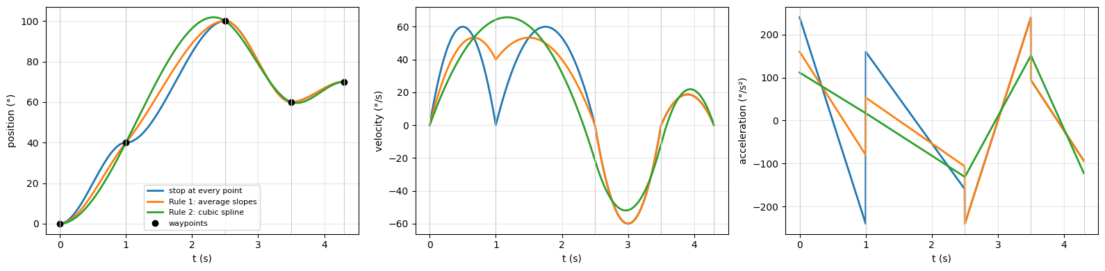
Stopping at every point brings the velocity to zero at each via point. Rule 1 keeps moving through 40°, where the joint continues upward, and stops at 100° and at 60°, where it turns back. The spline keeps the acceleration continuous (no jumps at the vertical lines) and has by far the lowest peak acceleration, but it runs through every via point with some velocity, even where the joint turns back, so it overshoots: it climbs past 100° before coming down, and dips below 60° before rising to 70°. We will see what that means in space shortly.
8.4.2 Linear segments with parabolic blends
The trapezoid of Section 8.3 is a straight line in time with a parabola at each end. With more waypoints, keep that idea: move along each segment at constant velocity , and around each waypoint replace the corner between two segments by a parabolic blend, a period of constant acceleration centred on the waypoint time. At the first and last waypoints the velocity before (after) the motion is zero, so those blends are exactly the accelerate and decelerate phases of a trapezoid.
The trajectory starts exactly at and stops exactly at , but it does not pass through the via points. In the middle of blend it is off by
because during the half-blend before the waypoint it is still on the incoming line but has started to turn. With the shortest blend the acceleration limit allows, , the miss is : a fast change of direction with a low acceleration limit cuts the corner the most.
Planning from the limits. For several joints:
Cruise as fast as the slowest joint allows: .
Blend as quickly as the slowest joint allows, with one blend time per waypoint for all joints: . Because all joints blend together, the corner of the joint-space path is replaced by one smooth curve.
The two blends of a segment must not overlap, . If they do, the segment is too short to reach its cruise speed: lengthen (which lowers and shortens the blends) until they fit.
The total time is . Industrial robot languages offer the same choice for every waypoint: an exact stop, or a “fly-by” point that the robot only passes near (ABB calls the allowed distance a zone, KUKA approximate positioning, Universal Robots a blend radius).
def parabolic_blends(points, durations, blend_times):
    # Linear segments with parabolic blends through waypoints (n+1, dof); segment durations (n,);
    # blend times (n+1,), one per waypoint, the first and last being the start and stop.
    # Returns (traj, T) with traj(t) -> (q, qd, qdd); the motion starts at t = 0.
    P, Tk, tb = np.atleast_2d(points).astype(float), np.asarray(durations, float), np.asarray(blend_times, float)
    n, zero = len(Tk), np.zeros(P.shape[1])
    t_knots = np.r_[0.0, np.cumsum(Tk)]                                   # waypoint times
    V = np.vstack([zero, np.diff(P, axis=0) / Tk[:, None], zero])         # V[k]: velocity before waypoint k, V[k+1]: after
    dV = V[1:] - V[:-1]
    acc = np.divide(dV, tb[:, None], out=np.zeros_like(dV), where=tb[:, None] > 0)   # constant acceleration in blend k
                                                                          # (no blend where the velocity does not change)
    assert np.all((tb[:-1] + tb[1:]) / 2 <= Tk + 1e-9), 'blends overlap: lengthen the segments'
    t_start, t_end = -tb[0] / 2, t_knots[-1] + tb[-1] / 2                 # the first blend starts before waypoint 0

    def traj(t):
        t = t + t_start
        if t <= t_start:                                                  # before the start: at rest at the first point
            return P[0].copy(), zero, zero
        if t >= t_end:                                                    # after the end: at rest at the last point
            return P[-1].copy(), zero, zero
        for k in range(n + 1):
            if abs(t - t_knots[k]) <= tb[k] / 2:                         # inside blend k
                tau = t - (t_knots[k] - tb[k] / 2)
                return P[k] - V[k] * tb[k] / 2 + V[k] * tau + 0.5 * acc[k] * tau**2, V[k] + acc[k] * tau, acc[k]
        k = min(max(np.searchsorted(t_knots, t, side='right') - 1, 0), n - 1)
        return P[k] + V[k + 1] * (t - t_knots[k]), V[k + 1], zero          # on the straight part of segment k
    return traj, t_end - t_start


def plan_blends(points, v_max, a_max):
    # Segment durations and blend times from the speed and acceleration limits (steps 1 to 3 above)
    P = np.atleast_2d(points).astype(float)
    zero = np.zeros((1, P.shape[1]))
    Tk = np.max(np.abs(np.diff(P, axis=0)) / v_max, axis=1)              # 1. cruise at the speed limit
    for _ in range(100):
        V = np.vstack([zero, np.diff(P, axis=0) / Tk[:, None], zero])
        tb = np.max(np.abs(np.diff(V, axis=0)) / a_max, axis=1)           # 2. shortest common blend
        need = (tb[:-1] + tb[1:]) / 2
        if np.all(Tk >= need * (1 - 1e-9)):
            break
        Tk = np.where(need > Tk, np.sqrt(Tk * need) * 1.0001, Tk)         # 3. lengthen segments whose blends overlap
    return Tk, tb


Tk, tb = plan_blends(wp, 90.0, 360.0)                                    # the five waypoints above: 90°/s, 360°/s²
traj, T = parabolic_blends(wp, Tk, tb)
t, q, qd, qdd = sample(traj, T, 3001)

fig, axes = plt.subplots(1, 2, figsize=(14, 4))
t_wp = np.r_[0, np.cumsum(Tk)] + tb[0] / 2                               # waypoint times on the new clock
axes[0].plot(t_wp, wp[:, 0], 'k--o', lw=1, ms=6, label='waypoints, joined by straight lines')
axes[0].plot(t, q[:, 0], lw=2, label='parabolic blends')
axes[1].plot(t, qd[:, 0], lw=2)
for ax, label in zip(axes, ('position (°)', 'velocity (°/s)')):
    ax.set_xlabel('t (s)'); ax.set_ylabel(label); ax.grid(alpha=0.3)
axes[0].legend(); plt.tight_layout(); plt.show()

V = np.vstack([[0.0], np.diff(wp, axis=0) / Tk[:, None], [0.0]])
print(f'Total time {T:.3f} s, peak speed {np.abs(qd).max():.1f}°/s, peak acceleration {np.abs(qdd).max():.1f}°/s²')
print(f"\n{'via point':>9} {'θ_k (°)':>8} {'at the blend centre (°)':>24} {'miss':>7} {'(V_k - V_k-1) t_b / 8':>23}")
for k in range(1, len(wp) - 1):
    reached = traj(t_wp[k])[0][0]
    print(f'{k:9d} {wp[k, 0]:8.1f} {reached:24.2f} {reached - wp[k, 0]:7.2f} {(V[k + 1, 0] - V[k, 0]) * tb[k] / 8:23.2f}')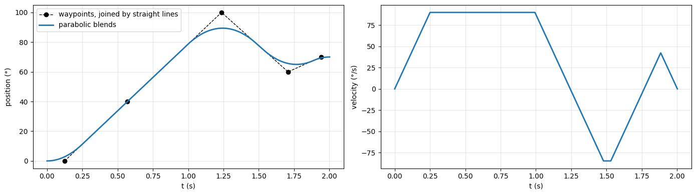
Total time 2.002 s, peak speed 90.0°/s, peak acceleration 360.0°/s²

via point  θ_k (°)  at the blend centre (°)    miss   (V_k - V_k-1) t_b / 8
        1     40.0                    40.00    0.00                    0.00
        2    100.0                    89.39  -10.61                  -10.61
        3     60.0                    65.62    5.62                    5.62
The dashed polyline is the constant-velocity reference: each waypoint is drawn at its waypoint time, , shifted by half the first blend so the motion starts at . The trajectory starts exactly at the first point and stops exactly at the last one; its first and last blends are the trapezoid’s acceleration and deceleration. In between it cruises at the 90°/s limit on the long segments and rounds every corner with a 360°/s² blend. Via point 1 is not a corner at all (both neighbouring segments run at the speed limit, upward), so it is passed exactly. At the other via points the miss is exactly : at the 100° peak the joint turns around more than 10° early, the price of not stopping there.
8.4.3 Comparing the methods on a 2R arm
Now the shape in space. The planar 2R arm works in a vertical plane, with its base at the
origin and a table at m. It must take a block from to
, lifting it through the via points above and
above . The waypoints are converted to joint angles with ik_2R on the
elbow-up branch (elbow=-1), which keeps the elbow well above the table, and each method
interpolates the joint angles. The cubic methods use the segment durations 1.0, 1.5 and 1.0 s; the blends are
planned from the limits rad/s and rad/s².
xy_A, xy_A_up, xy_B_up, xy_B = (1.35, 0.1), (1.35, 0.7), (0.55, 0.7), (0.55, 0.1)
TABLE_Y = 0.05
Q_wp = np.array([ik_2R(*p, elbow=-1) for p in (xy_A, xy_A_up, xy_B_up, xy_B)])   # elbow up
durs_2R = np.array([1.0, 1.5, 1.0])
V_LIM_2R, A_LIM_2R = 2.0, 6.0                                            # rad/s, rad/s²

plans_2R = {name: cubic_segments(Q_wp, durs_2R, V) for name, V in [
    ('stop at every point (cubics)', np.zeros_like(Q_wp)),
    ('Rule 1: average slopes', via_velocities_average(Q_wp, durs_2R)),
    ('Rule 2: cubic spline', via_velocities_spline(Q_wp, durs_2R))]}
plans_2R['parabolic blends'] = parabolic_blends(Q_wp, *plan_blends(Q_wp, V_LIM_2R, A_LIM_2R))

fig, axes = plt.subplots(1, 2, figsize=(15, 5.5), gridspec_kw={'width_ratios': [1, 1.2]})
ax = axes[0]
ax.plot(*np.array([xy_A, xy_A_up, xy_B_up, xy_B]).T, 'k--o', lw=1, ms=6, label='waypoints')
for name, (traj, T) in plans_2R.items():
    t, q, qd, qdd = sample(traj, T, 1501)
    ax.plot(*fk_2R(q)[1].T, lw=2, label=name)
    axes[1].plot(t / T, qd[:, 0], lw=2, label=name)
draw_2R(ax, Q_wp[0], alpha=0.25)
ax.axhline(TABLE_Y, color='k', lw=2); ax.text(1.5, TABLE_Y + 0.01, 'table', va='bottom')
ax.set_aspect('equal'); ax.grid(alpha=0.3); ax.set_xlim(-0.1, 1.75); ax.set_ylim(-0.05, 1.2)
ax.legend(fontsize=8, loc='upper left'); ax.set_title('Tip paths')
axes[1].set_xlabel('t / T (each method on its own duration)'); axes[1].set_ylabel('θ̇₁ (rad/s)')
axes[1].grid(alpha=0.3); axes[1].set_title('Shoulder velocity')
plt.tight_layout(); plt.show()

print(f'Time to run the same waypoints within v_max = {V_LIM_2R} rad/s and a_max = {A_LIM_2R} rad/s²:')
stops = sum(sync_trapezoid(Q_wp[k], Q_wp[k + 1], V_LIM_2R, A_LIM_2R)[0] for k in range(3))
print(f"  {'stop at every point (fastest trapezoids)':<42} {stops:5.2f} s")
for name, (traj, T) in plans_2R.items():
    t, q, qd, qdd = sample(traj, T, 3001)
    k = max(np.abs(qd).max() / V_LIM_2R, np.sqrt(np.abs(qdd).max() / A_LIM_2R))   # scaling law, Section 8.1
    print(f"  {name:<42} {T * k:5.2f} s")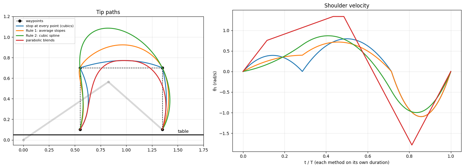
Time to run the same waypoints within v_max = 2.0 rad/s and a_max = 6.0 rad/s²:
  stop at every point (fastest trapezoids)    2.11 s
  stop at every point (cubics)                2.99 s
  Rule 1: average slopes                      2.99 s
  Rule 2: cubic spline                        2.65 s
  parabolic blends                            1.59 s
Three lessons:
Smoothest in time is not best in space. The spline has the smoothest joint motion, yet its tip path swings far above the via points (to m) and out past near the pick point, where a neighbouring object would be hit. Rule 1 bulges less. The parabolic blends rise no higher than stopping at every point (both reach m on the carry), but they cut the corners hard: with these limits the tip passes 8.6 cm from and 17.7 cm from (the explorer below prints these distances).
Even “stop at every point” is not straight. All four methods interpolate joint angles, so the vertical lifts and descents come out curved, most of all near , close to the base (Section 8.5 explains why and shows how to get straight lines).
Not stopping is faster. Within the same limits, the blends need about a quarter less time than the fastest stop-at-every-point trapezoids (1.59 s vs 2.11 s), because they keep moving through the corners and cruise at the speed limit. The cubic methods are slower still: their hand-picked segment durations, stretched by the scaling law until the limits hold, do not use the limits well.
Whatever the method, check the path with forward kinematics before running it, as we did here: plot the gripper path and compare it with the table and the objects around it.
Explore the blends. The sliders set the limits. Lower the acceleration limit and watch the corners round off more; raise the speed limit and the corners round off more too, because faster segments need longer blends to turn.
def explore_blends():
    def _view(v_max=2.0, a_max=6.0):
        Tk, tb = plan_blends(Q_wp, v_max, a_max)
        traj, T = parabolic_blends(Q_wp, Tk, tb)
        t, q, _, _ = sample(traj, T, 1501)
        tip = fk_2R(q)[1]
        fig, ax = plt.subplots(figsize=(7, 5))
        ax.plot(*np.array([xy_A, xy_A_up, xy_B_up, xy_B]).T, 'k--o', lw=1, ms=6)
        ax.plot(*tip.T, lw=2.5, color='tab:red')
        ax.axhline(TABLE_Y, color='k', lw=2)
        miss = [np.min(np.linalg.norm(tip - np.array(p), axis=1)) for p in (xy_A_up, xy_B_up)]
        ax.set_title(f'T = {T:.2f} s;  tip passes {100 * miss[0]:.1f} cm from A\', {100 * miss[1]:.1f} cm from B\'')
        ax.set_aspect('equal'); ax.grid(alpha=0.3); ax.set_xlim(0.2, 1.7); ax.set_ylim(0.0, 1.0)
        plt.show()

    interact(_view,
             v_max=FloatSlider(value=2.0, min=0.5, max=4.0, step=0.1, description='v_max (rad/s)'),
             a_max=FloatSlider(value=6.0, min=1.0, max=20.0, step=0.5, description='a_max (rad/s²)'))


explore_blends()8.4.4 Where the robot must stop
Not stopping saves time, but some waypoints still need the arm at rest:
Grasp and release. The gripper closes or opens while the arm holds still; a block grabbed on the move slides or tips.
Contact and precise placement. Setting a block on a stack, or anything that touches, ends at rest, ideally with a short, slow final approach.
Every other waypoint (above the pick, above the goal, points that steer around obstacles) can be a via point.
When a waypoint becomes a via point, the path near it changes: blends cut the corner (Section 8.4.2) and cubics can bulge (Section 8.4.3). If the via point was there to give clearance, for example to lift a block 6 cm before moving sideways, raise it by the amount the corner is cut, or plan the blend with a smaller speed or a larger acceleration, and check the result with forward kinematics.
Key Takeaways — Section 8.4
Stop only where the task needs it (grasp, release, contact); pass every other waypoint as a via point.
Cubic segments with via velocities pass exactly through the points with continuous velocity. Rule 1: average the neighbouring slopes, or 0 where the joint turns back. Rule 2 (cubic spline): a tridiagonal system that also makes the acceleration continuous.
Linear segments with parabolic blends: cruise between points, blend around them; the miss at a via point is , or with the shortest blend. Plan from and from , with one blend time for all joints.
Smoothest in time is not best in space: always check the gripper path with forward kinematics.
8.5 Straight-Line Trajectories in Task Space
8.5.1 Joint space is not task space
Every trajectory so far interpolates joint angles, and the gripper follows whatever curve the forward kinematics makes of them. Section 8.4.3 showed curved “vertical” lifts on the 2R arm. On the SO-ARM101, the same happens for the two moves of a pick and place, with the gripper pointing straight down:
the descent from 6 cm above the pick spot down to the grasp height, and
the carry from 6 cm above the pick spot to 6 cm above the place spot.
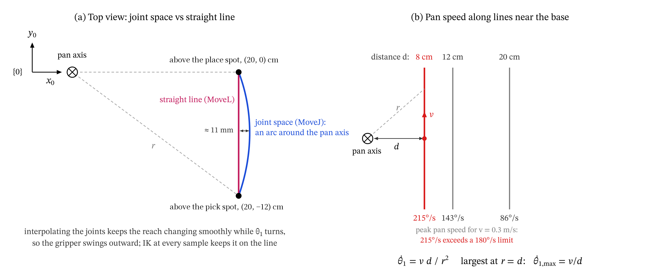
Figure 8.4 — SO-ARM101 seen from above. (a) Interpolating the joints swings the gripper in an arc around the pan axis (blue); a straight line needs IK at every sample (red). (b) The same gripper speed v on lines closer to the pan axis needs a faster pan joint: θ̇1,max = v/d (Section 8.5.3).
Figure 8.4(a) shows the carry. The cell runs both moves as joint-space cubics and measures how far the gripper point strays from the straight line between the ends.
def gripper_path(traj, T, n=200):
    # Gripper point o_e along a trajectory, from the forward kinematics; (n, 3) array
    return np.array([so101.fk(traj(t)[0])[:3, 3] for t in np.linspace(0, T, n)])


def distance_from_line(points, a, b):
    # Distance of each point from the straight line through a and b
    u = (b - a) / np.linalg.norm(b - a)
    d = points - a
    return np.linalg.norm(d - np.outer(d @ u, u), axis=1)


q_above_pick, q_grasp = so101_top_down(PICK_XY, Z_GRASP + LIFT), so101_top_down(PICK_XY, Z_GRASP)
q_above_place = so101_top_down(PLACE_XY, Z_GRASP + LIFT)
joint_moves = {'descent': cubic_segments([q_above_pick, q_grasp], [1.0], np.zeros((2, 5))),
               'carry': cubic_segments([q_above_pick, q_above_place], [1.0], np.zeros((2, 5)))}

fig, axes = plt.subplots(1, 2, figsize=(14, 4.8))
for name, (traj, T) in joint_moves.items():
    path = gripper_path(traj, T)
    off = distance_from_line(path, path[0], path[-1])
    print(f'joint-space {name:<8}: the gripper point strays up to {1000 * off.max():5.1f} mm from the straight line')
desc = gripper_path(*joint_moves['descent'])
axes[0].plot(1000 * np.hypot(*(desc[:, :2] - desc[-1, :2]).T), 100 * desc[:, 2], lw=2, label='joint-space cubic')
axes[0].axvline(0, color='k', ls='--', label='straight down')
axes[0].set_xlabel('horizontal distance from the grasp point (mm)'); axes[0].set_ylabel('height (cm)')
axes[0].set_title('Descent at the pick spot, seen from the side')
carry = gripper_path(*joint_moves['carry'])
axes[1].plot(100 * carry[:, 0], 100 * carry[:, 1], lw=2, label='joint-space cubic')
axes[1].plot(100 * carry[[0, -1], 0], 100 * carry[[0, -1], 1], 'k--', label='straight line')
axes[1].plot(100 * geo.xp, 0, 'k+', ms=12); axes[1].text(100 * geo.xp + 0.5, 0.5, 'pan axis')
axes[1].set_xlabel('x (cm)'); axes[1].set_ylabel('y (cm)'); axes[1].set_aspect('equal')
axes[1].set_title('Carry, seen from above')
for ax in axes:
    ax.grid(alpha=0.3); ax.legend()
plt.tight_layout(); plt.show()
joint-space descent : the gripper point strays up to 3.0 mm from the straight line
joint-space carry : the gripper point strays up to 11.3 mm from the straight line
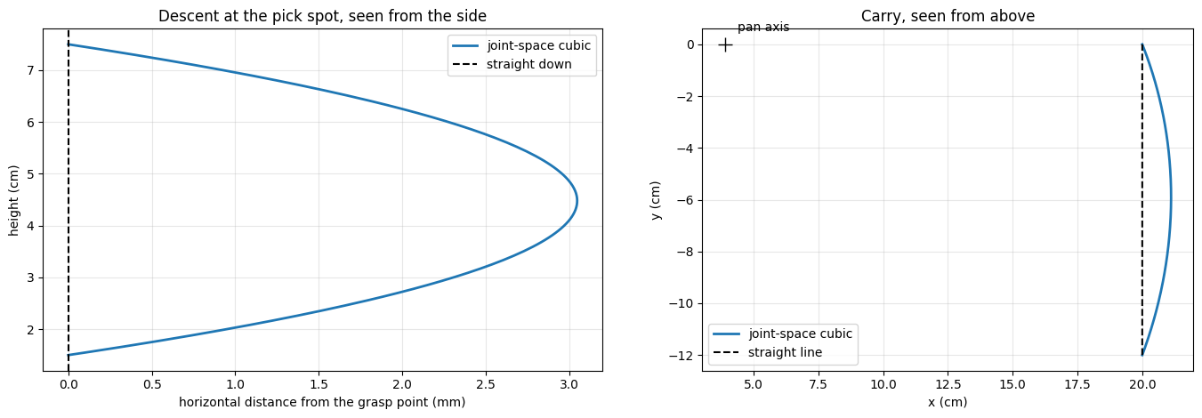
The carry swings in an arc around the pan axis: interpolating the joints keeps the reach roughly constant while the pan joint turns. The descent drifts a few millimetres sideways and comes back. A few millimetres matter when the fingers must come down around a 1-inch block with a few millimetres to spare.
8.5.2 Interpolating the gripper position
To move the gripper along a straight line, interpolate the gripper position and let the inverse kinematics find the joint angles at every instant:
Any time scaling of Sections 8.2 and 8.3 can be used for . The orientation is interpolated the same way. For the SO-ARM101 that is just the pitch, (constant here). For a full orientation, turn about one fixed axis: if is the axis-angle form (Section 4.3.3) of the rotation from the start to the goal, use , which is the same as quaternion SLERP.
Three checks, at every sample, not just at the ends:
Reachable: every point of the line must be inside the workspace.
Within the joint limits.
Same branch: the IK must keep choosing the same solution (elbow up, facing the target). Switching branches mid-line makes the joints jump.
def so101_line(p0, pf, T, phi=PHI_DOWN):
    # Straight line of the gripper point from p0 to pf in T seconds, cubic time scaling, constant pitch.
    # Returns traj(t) -> (q, qd, qdd); velocities and accelerations by finite differences.
    p0, pf = np.asarray(p0, float), np.asarray(pf, float)
    a = cubic_coefficients(0.0, 1.0, T)

    def q_at(t):
        q = so101_ik(p0 + poly_eval(a, min(max(t, 0.0), T))[0] * (pf - p0), phi)
        assert q is not None and so101.within_limits(q), f'line leaves the workspace at t = {t:.3f} s'
        return q

    def traj(t, h=1e-4):
        q_minus, q_now, q_plus = q_at(t - h), q_at(t), q_at(t + h)
        return q_now, (q_plus - q_minus) / (2 * h), (q_plus - 2 * q_now + q_minus) / h**2
    return traj


p_above_pick, p_grasp = np.array([*PICK_XY, Z_GRASP + LIFT]), np.array([*PICK_XY, Z_GRASP])
p_above_place = np.array([*PLACE_XY, Z_GRASP + LIFT])
line_moves = {'descent': (so101_line(p_above_pick, p_grasp, 1.0), 1.0),
              'carry': (so101_line(p_above_pick, p_above_place, 1.0), 1.0)}

for name in ('descent', 'carry'):
    for kind, (traj, T) in (('joint space', joint_moves[name]), ('straight line', line_moves[name])):
        t, q, qd, qdd = sample(traj, T, 401)
        path = gripper_path(traj, T)
        off = distance_from_line(path, path[0], path[-1]).max()
        print(f'{name:<8} {kind:<14} off the line {1000 * off:6.2f} mm   peak joint speeds (°/s): '
              + ' '.join(f'{v:6.1f}' for v in np.degrees(np.abs(qd).max(axis=0)[:4])))
descent joint space off the line 3.05 mm peak joint speeds (°/s): 0.0 6.3 30.2 36.6
descent straight line off the line 0.00 mm peak joint speeds (°/s): 0.0 9.8 32.1 36.5
carry joint space off the line 11.27 mm peak joint speeds (°/s): 55.0 30.6 36.0 5.4
carry straight line off the line 0.00 mm peak joint speeds (°/s): 57.7 39.6 47.8 9.3
Both straight lines are straight to within a hundredth of a millimetre (what remains is the 0.01 mm sideways offset that Section 7.4.5 removes). For the same 1-second carry the straight line asks more of the shoulder and elbow, which must pull the gripper in toward the base and push it out again instead of letting it swing around in an arc.
8.5.3 Joint speeds along a line, and choosing 
Differentiating gives the gripper velocity , and the joint velocities follow from the inverse velocity relation of Section 6.6.1,
A straight-line trajectory is the resolved-rate motion of Chapter 6 with a time-scaled velocity. Near a singularity is nearly singular, and even a slow gripper needs very fast joints (Path B in Section 6.6.1). For the SO-ARM101 there is a simple special case: a horizontal line that passes at distance from the pan axis, travelled at speed , turns the pan joint at
Lines that pass close to the base need a fast pan joint (Figure 8.4(b)). The cell checks the formula on three parallel 20 cm lines, each run in 1 s, 3 cm above the grasp height.
print(f"{'distance d (cm)':>16} {'peak gripper speed (m/s)':>25} {'peak pan speed (°/s)':>21} {'v/d (°/s)':>10}")
for d in (0.20, 0.12, 0.08):
    x = geo.xp + d
    traj = so101_line([x, -0.10, Z_GRASP + 0.03], [x, 0.10, Z_GRASP + 0.03], 1.0)
    t, q, qd, qdd = sample(traj, 1.0, 801)
    v_peak = 1.5 * 0.20 / 1.0                                            # cubic: 1.5 Δ/T
    print(f'{100 * d:16.0f} {v_peak:25.2f} {np.degrees(np.abs(qd[:, 0]).max()):21.1f} {np.degrees(v_peak / d):10.1f}')
distance d (cm) peak gripper speed (m/s) peak pan speed (°/s) v/d (°/s)
              20                      0.30                  85.9       85.9
              12                      0.30                 143.2      143.2
               8                      0.30                 214.9      214.9
The formula matches the simulated peaks exactly. The same gripper speed that needs 86°/s of pan speed 20 cm from the axis needs 215°/s at 8 cm, more than our 180°/s limit: that line must be run more slowly, or moved away from the base.
Choosing for a line. The joint speeds of a straight line change along it, so there is no closed-form as in Section 8.2.4. The scaling law of Section 8.1 still holds, because the shape of the motion does not change when does: sample the trajectory once, find the peak joint speed and acceleration, and stretch it by .
def min_duration(make_traj, v_max, a_max, T_try=1.0, n=401):
    # Shortest T for a trajectory family make_traj(T) -> traj, from one trial run and the scaling law
    t, q, qd, qdd = sample(make_traj(T_try), T_try, n)
    return T_try * max(np.abs(qd).max() / v_max, np.sqrt(np.abs(qdd).max() / a_max))


for name, (p0, pf) in {'descent': (p_above_pick, p_grasp), 'carry': (p_above_pick, p_above_place)}.items():
    T_line = min_duration(lambda T: so101_line(p0, pf, T), V_MAX, A_MAX)
    T_joint = sync_trapezoid(so101_top_down(p0[:2], p0[2]), so101_top_down(pf[:2], pf[2]), V_MAX, A_MAX)[0]
    t, q, qd, qdd = sample(so101_line(p0, pf, T_line), T_line, 401)
    print(f'{name:<8}: straight line (cubic timing) {T_line:.3f} s, peak joint speed {np.degrees(np.abs(qd).max()):5.1f}°/s, '
          f'peak acceleration {np.degrees(np.abs(qdd).max()):5.1f}°/s²   |   joint-space trapezoid {T_joint:.3f} s')
descent : straight line (cubic timing) 0.489 s, peak joint speed 74.5°/s, peak acceleration 720.0°/s² | joint-space trapezoid 0.368 s
carry : straight line (cubic timing) 0.658 s, peak joint speed 87.7°/s, peak acceleration 720.0°/s² | joint-space trapezoid 0.451 s
The straight line costs some time: it uses cubic timing (Section 8.3.2: a trapezoid needs about 15% less time), and its joint speeds vary along the line, so the limit is reached only at one point. Near the table, where the path matters, that is usually worth it.
8.5.4 Joint space or task space?
| Joint-space path | Straight line in task space | |
|---|---|---|
| Industrial name | MoveJ (joint move) | MoveL (linear move) |
| Gripper path | a curve (an arc around the base for a carry) | a straight line |
| Needs | IK at the two ends only | IK at every sample, all reachable, same branch |
| Joint speeds | set directly by the time scaling | vary along the line; large near singularities and near the pan axis |
| Speed | fastest for a given limit | slower |
| Use for | large moves through free space | approaching, grasping, lifting, placing |
Key Takeaways — Section 8.5
Interpolating joints moves the gripper along a curve: the SO-ARM101 carry swings in an arc around the pan axis, and a “vertical” descent drifts sideways by millimetres.
Straight line: , ; orientation about a fixed axis (axis-angle, SLERP). Check reachability, limits and branch at every sample.
Joint speeds: ; large near singularities. For the SO-ARM101 pan joint, .
Choose by sampling once and applying the scaling law. Straight lines near objects, joint-space moves through free space.
8.6 From a Trajectory to Motor Commands
A trajectory is a function , but a servo only accepts goal positions. Three layers turn one into the other:
| Layer | Where | How often | What it does |
|---|---|---|---|
| Planner | your program | once per move | chooses the path and the timing (Sections 8.1 to 8.5) |
| Sampler | your program | every (for example 20 ms) | evaluates and sends it as the goal position of each servo |
| Servo | inside each motor | much faster | its own feedback loop drives the motor toward the latest goal |
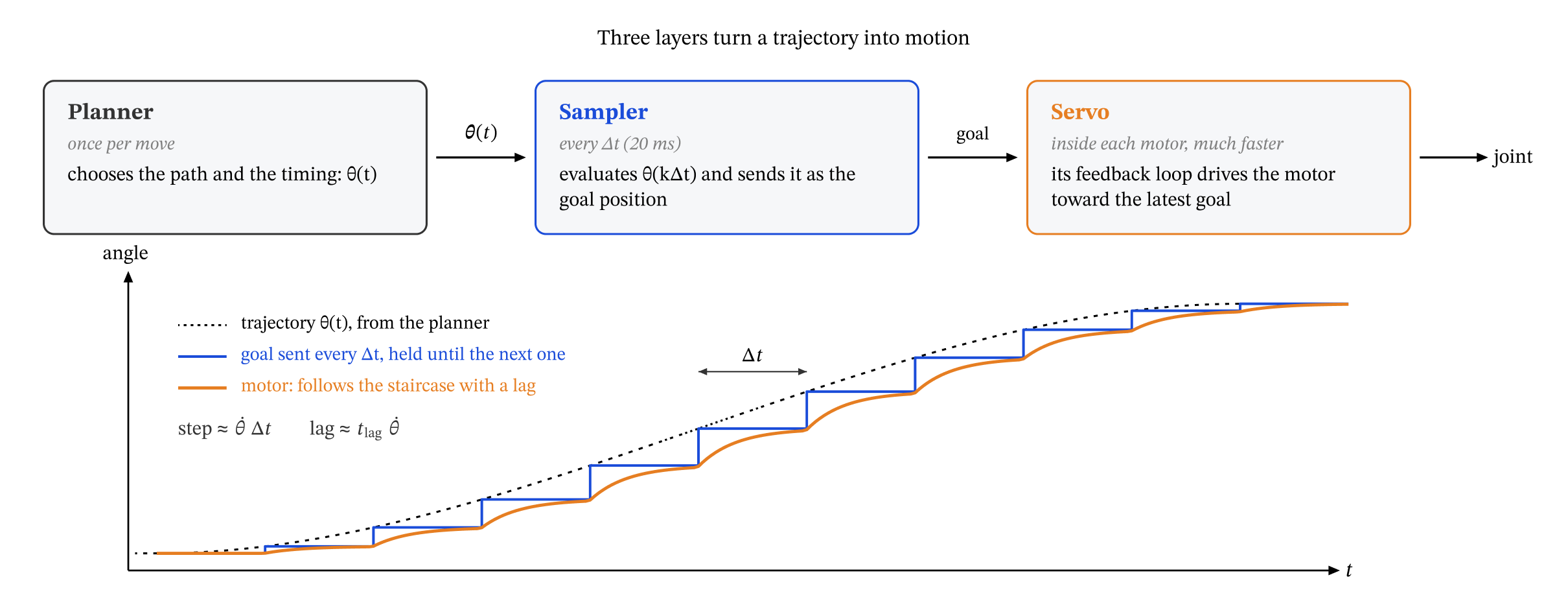
Figure 8.5 — From a trajectory to motion. The planner computes θ(t); the sampler sends θ(kΔt) as the goal every Δt and holds it; the servo follows that staircase with a lag of about tlag θ̇.
Sampling. Between samples the goal is held constant, so the servo sees a staircase that follows the trajectory. Each step is about : at 100°/s, 2° at 50 Hz but 10° at 10 Hz. Coarser steps make the motion jerkier and add delay, because on average the goal is already old.
Tracking. A position servo needs an error to make torque, so it lags behind a moving goal. A simple model: the servo closes the gap with a time constant , . For a goal moving at speed the error settles at . The cell uses ms, about what the SO-101’s simulated servos show, and a 75° move in 1 s.
def servo_response(trajectory_q, T, dt_sample, t_lag=0.015, t_after=0.4, h=1e-4):
    # Simple servo model: the goal is sampled every dt_sample and held; the motor follows with time constant t_lag.
    t = np.arange(0, T + t_after, h)
    goal = np.array([trajectory_q(np.floor(ti / dt_sample) * dt_sample) for ti in t])   # sample and hold
    motor = np.zeros_like(t)
    motor[0] = goal[0]
    for k in range(1, len(t)):
        motor[k] = motor[k - 1] + h * (goal[k - 1] - motor[k - 1]) / t_lag
    exact = np.array([trajectory_q(ti) for ti in t])
    return t, goal, motor, exact


D, T = 75.0, 1.0
linear_q = lambda t: D * min(max(t / T, 0.0), 1.0)
cubic_q = lambda t: poly_eval(cubic_coefficients(0.0, D, T), min(max(t, 0.0), T))[0]

fig, axes = plt.subplots(1, 2, figsize=(15, 4.2))
print(f"{'trajectory':<10} {'rate':>6} {'peak error (°)':>15} {'error at t = T (°)':>19}")
for name, traj_q, ls in (('linear', linear_q, '--'), ('cubic', cubic_q, '-')):
    for hz in (50, 10):
        t, goal, motor, exact = servo_response(traj_q, T, 1 / hz)
        err = exact - motor
        axes[0].plot(t, err, ls, lw=1.8, label=f'{name}, {hz} Hz')
        print(f'{name:<10} {hz:4d} Hz {np.abs(err[t <= T]).max():15.2f} {err[np.argmin(np.abs(t - T))]:19.2f}')
t, goal, motor, exact = servo_response(cubic_q, T, 1 / 10)
axes[1].plot(t, exact, 'k:', lw=1.5, label='trajectory')
axes[1].plot(t, goal, lw=1.5, label='goal sent at 10 Hz (held)')
axes[1].plot(t, motor, lw=2, label='motor')
axes[0].set_ylabel('trajectory − motor (°)'); axes[0].set_title('Tracking error, simple servo model')
axes[1].set_ylabel('angle (°)'); axes[1].set_title('Cubic at 10 Hz: the staircase'); axes[1].set_xlim(0.3, 0.7); axes[1].set_ylim(10, 65)
for ax in axes:
    ax.set_xlabel('t (s)'); ax.grid(alpha=0.3); ax.legend(fontsize=8)
plt.tight_layout(); plt.show()
trajectory rate peak error (°) error at t = T (°)
linear 50 Hz 2.03 2.03
linear 10 Hz 7.52 7.51
cubic 50 Hz 3.05 0.20
cubic 10 Hz 11.12 2.11
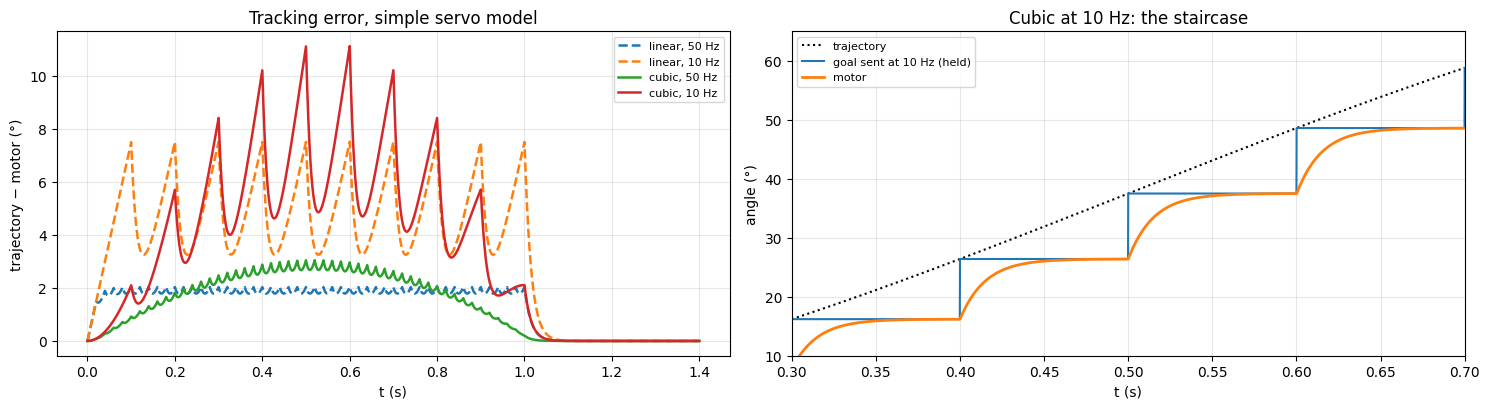
At 50 Hz the model shows the pattern a real servo shows. The linear trajectory’s error jumps as soon as the move starts, and the motor is still 2° behind, and still moving, at . The cubic’s error grows and shrinks with its speed: its peak is larger, because its peak speed is 1.5 times linear’s, but it comes in the middle of the move, and at the motor is almost on target and at rest. (This first-order model leaves out the overshoot a real servo shows when a linear move starts, which makes linear’s error at the start even larger.)
At 10 Hz the errors are several times larger: just before each new goal arrives, the goal is a full sample period old, so the error grows by up to (7.5° at 75°/s), and the motor visibly follows a staircase.
The servo’s own profile. Sent a single goal angle, an STS3215 servo moves there along its own trapezoidal velocity profile. When the sampler sends a new goal every 20 ms, each goal is only a step of a degree or two, and the built-in profile acts on those small steps; it no longer shapes the whole move, as long as its acceleration setting is high (LeRobot sets it high when it connects). Some servos also accept a move time with each goal, which gives a timed, smooth move from a single command. That is enough for a point-to-point joint move, but the profile shape is fixed by the servo, and a single command per move cannot follow a straight line in task space or pass a via point without stopping. That is why the trajectories of this chapter are streamed from the computer.
Key Takeaways — Section 8.6
Planner (once per move), sampler (every , sends goal positions), servo (fast internal loop).
Sampling holds each goal for : steps of , and about of extra delay.
A position servo lags by roughly : smooth trajectories keep that error small at the start and the end of a move.
A servo’s built-in profile handles one goal at a time; streaming lets the computer choose the shape, the path and the via points.
8.7 Putting It Together: A Fast Pick and Place on the SO-ARM101
We now move a block from the pick spot, cm, to the place spot, cm, with the gripper pointing straight down and a 6 cm lift, and compare three plans. Each starts and ends 6 cm above a spot, and each spends 0.5 s on closing and 0.5 s on opening the gripper.
Fixed times: every move takes a fixed, generous time (1 to 2.5 s), with a hold of 0.5 to 1 s after it.
Stop at every waypoint, as fast as the limits allow: a synchronized trapezoid (Section 8.3.3) for each move.
Via points: the descent to the block and the final retreat are trapezoids, but lift, carry and lower form one blended trajectory through the two “above” points (Section 8.4.2), stopping only at the block and at the goal.
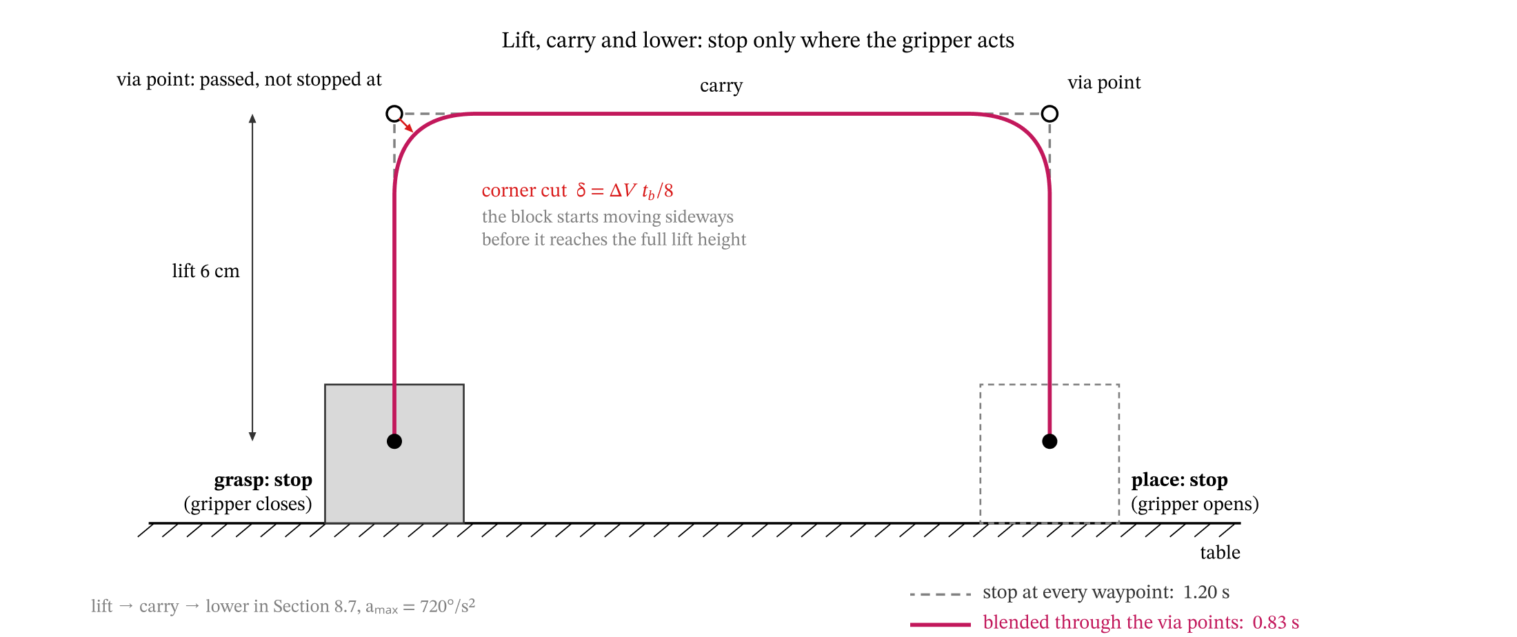
Figure 8.6 — Lift, carry and lower. The arm must stop at the grasp and the place, where the gripper acts; the points above them are via points. Blending through them (red) saves time but cuts the corners, so the block starts moving sideways before it is fully lifted. Times from the comparison below, with amax = 720°/s².
Figure 8.6 shows plan 3 next to stopping at every waypoint. Real limits are rarely the paper values: a block held in the gripper slips if the arm accelerates too hard. So the comparison runs for three acceleration limits.
GRIP_TIME = 0.5                                                          # s to close, and to open, the gripper
q_pick, q_pick_up = so101_top_down(PICK_XY, Z_GRASP), so101_top_down(PICK_XY, Z_GRASP + LIFT)
q_place, q_place_up = so101_top_down(PLACE_XY, Z_GRASP), so101_top_down(PLACE_XY, Z_GRASP + LIFT)

# Plan 1: fixed move and hold times (descend, close, lift, carry, lower, open, retreat)
T_plan1 = sum([1.5, 1.0, 1.5, 2.5, 1.5, 1.0, 1.5]) + sum([0.5, 1.0, 0.5, 0.5, 0.5, 1.0, 0.5])

print(f'Plan 1, fixed times: {T_plan1:.1f} s\n')
print(f"{'a_max (°/s²)':>12} {'plan 2: stop everywhere':>24} {'plan 3: via points':>19} {'saved':>7}   lift → carry → lower: stop vs blend")
for a_deg in (720, 360, 180):
    a_lim = np.radians(a_deg)
    T_down = sync_trapezoid(q_pick_up, q_pick, V_MAX, a_lim)[0]
    T_up = sync_trapezoid(q_place, q_place_up, V_MAX, a_lim)[0]
    transit_stop = sum(sync_trapezoid(a, b, V_MAX, a_lim)[0]
                       for a, b in [(q_pick, q_pick_up), (q_pick_up, q_place_up), (q_place_up, q_place)])
    transit_blend = parabolic_blends([q_pick, q_pick_up, q_place_up, q_place],
                                     *plan_blends([q_pick, q_pick_up, q_place_up, q_place], V_MAX, a_lim))[1]
    T2 = T_down + GRIP_TIME + transit_stop + GRIP_TIME + T_up
    T3 = T_down + GRIP_TIME + transit_blend + GRIP_TIME + T_up
    print(f'{a_deg:12d} {T2:22.2f} s {T3:17.2f} s {100 * (1 - T3 / T2):6.0f}%   {transit_stop:.2f} s vs {transit_blend:.2f} s')
Plan 1, fixed times: 15.0 s
a_max (°/s²) plan 2: stop everywhere plan 3: via points saved lift → carry → lower: stop vs blend
720 2.94 s 2.58 s 13% 1.20 s vs 0.83 s
360 3.75 s 3.23 s 14% 1.69 s vs 1.17 s
180 4.89 s 4.15 s 15% 2.40 s vs 1.66 s
Two lessons for a fast pick and place:
Time each move from the limits. Going from fixed, generous times to the fastest moves the limits allow is by far the largest gain: from 15 s per block to a few seconds.
Then remove the unnecessary stops. Blending through the two points above the block and above the goal saves about 30% of the lift-carry-lower time, and the saving grows as the acceleration limit is lowered, because each stop costs more when the arm must slow down gently.
The cost of not stopping is the corner. The cell plots the height of the gripper point against its horizontal distance from the block, for the blended plan and for the stop-everywhere plan.
P_transit = np.array([q_pick, q_pick_up, q_place_up, q_place])
fig, ax = plt.subplots(figsize=(10, 4.5))
for a_deg, color in ((720, 'tab:blue'), (180, 'tab:red')):
    traj, T = parabolic_blends(P_transit, *plan_blends(P_transit, V_MAX, np.radians(a_deg)))
    path = gripper_path(traj, T, 600)
    along = np.linalg.norm(path[:, :2] - path[0, :2], axis=1)
    ax.plot(100 * along, 100 * path[:, 2], lw=2, color=color, label=f'blended, a_max = {a_deg}°/s²')
    k = np.argmax(along > 0.01)
    print(f'a_max = {a_deg}°/s²: the gripper is 1 cm sideways from the block when only '
          f'{100 * (path[k, 2] - Z_GRASP):.1f} cm above the grasp height (of the 6 cm lift)')
stops = np.vstack([gripper_path(*cubic_segments(P_transit[k:k + 2], [1.0], np.zeros((2, 5)))) for k in range(3)])
ax.plot(100 * np.linalg.norm(stops[:, :2] - stops[0, :2], axis=1), 100 * stops[:, 2], 'k--', lw=1.5, label='stop at every waypoint')
ax.set_xlabel('horizontal distance from the block (cm)'); ax.set_ylabel('gripper height (cm)')
ax.set_aspect('equal'); ax.grid(alpha=0.3); ax.legend()
ax.set_title('Lift, carry and lower, seen from the side')
plt.tight_layout(); plt.show()
a_max = 720°/s²: the gripper is 1 cm sideways from the block when only 4.6 cm above the grasp height (of the 6 cm lift)
a_max = 180°/s²: the gripper is 1 cm sideways from the block when only 4.6 cm above the grasp height (of the 6 cm lift)
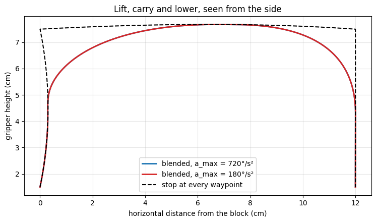
The blend rounds off the top corners, here by about 1.4 cm of the 6 cm lift: the block starts moving sideways before it is fully lifted. The amount does not depend on the acceleration limit in this plan, because the planner scales the segment speeds and the blends together. If neighbouring blocks or a growing stack need the full clearance, raise the via points by the amount cut, and check again.
For a fast pick and place, this is the recipe:
Compute every waypoint with IK from the block and goal positions (Chapter 7), and check it against the joint limits (the far spots need a tilted pitch, Section 7.4.4).
Decide which waypoints are stops (grasp, release, placing on a stack) and which are via points.
Time every move from measured speed and acceleration limits, not from guesses: trapezoids for moves that stop, blends through via points.
Use straight lines (Section 8.5) where the path near a block matters; joint-space moves elsewhere.
Check every gripper path with FK against the table, the waiting blocks and the stack, then simulate it before running it on the robot.
Chapter 8 Summary
Path vs trajectory: a trajectory is a path plus a time scaling . On a straight joint-space path every joint uses the same : . Stretching time by divides velocities by and accelerations by .
Polynomials: linear (velocity jumps), cubic (four conditions; rest to rest , peak , ), quintic (six conditions; , continuous acceleration). .
Trapezoid (LSPB): ; with , the fastest rest-to-rest move. Synchronize joints with , .
Via points: cubic segments with via velocities (average-slope rule, or the spline’s tridiagonal system for continuous acceleration), or linear segments with parabolic blends (miss ). Stop only where the task needs it, and check the path with FK.
Task space: for straight lines; grows near singularities (and near the pan axis, ).
Execution: sample every and stream goal positions; the servo lags by about .
| Method | Passes through the points | Stops at the points | Continuous | Chooses from limits |
|---|---|---|---|---|
| Linear | yes | yes | position | no (infinite acceleration) |
| Cubic, rest to rest | yes | yes | velocity | formula |
| Quintic, rest to rest | yes | yes | acceleration | formula |
| Trapezoid | yes | yes | velocity | yes, fastest |
| Cubic segments, average-slope velocities | yes | only where a joint turns back | velocity | scaling law |
| Cubic spline | yes | no (except the ends) | acceleration | scaling law |
| Parabolic blends | no (cuts corners) | no (except the ends) | velocity | yes |
| Straight line in task space | yes, along a line | yes | as its | sample + scaling law |
Practice problems
A joint moves from to in s, starting at rest and ending at /s. Find the cubic coefficients by hand and check them with
cubic_coefficients. Does the joint overshoot ?Show that the rest-to-rest cubic has peak velocity and end accelerations , and that the rest-to-rest quintic has peak velocity .
Trapezoid: a joint must move with /s and /s². Find and . Is the profile a trapezoid or a triangle? Then find and the cruise speed for a move of exactly s with /s².
Two joints move . Joint 1 has limits /s and /s²; joint 2, /s and /s². Which joint sets the pace of a synchronized trapezoid, and what is ?
Via points: one joint passes at s. Find the via velocities with the average-slope rule and with the spline (solve the system by hand), and compare with
via_velocities_averageandvia_velocities_spline.A blend turns a joint from /s to /s with /s². How long is the blend, and by how much does the joint miss the via point?
SO-ARM101: a straight carry passes 6 cm from the pan axis with a peak gripper speed of 0.25 m/s. What pan speed does it need, and is it within /s? What could you change?
Extend Section 8.7 to stacking six blocks into a pyramid (three on the table, two on them, one on top): list the waypoints for one block, mark which are stops, and estimate the total time with the plan-3 numbers. Which waypoints need extra clearance as the pyramid grows?