In Chapter 3 we found where the tip of a 2R arm is by drawing triangles and using trigonometry. That works for two links in a plane, but it gets messy fast: add a third link, or lift the arm into 3D, and you have to start the geometry over.
This chapter gives us a systematic tool instead. The idea:
Glue a coordinate frame to every link.
Describe each frame only relative to the frame one step before it — a small, local question.
Store each answer as one matrix, the homogeneous transformation matrix (HTM), and chain the steps together by plain matrix multiplication.
Chapter 5 turns this into a recipe for the forward kinematics of any robot arm, and Chapter 6 reuses the same frames to get velocities.
After this chapter you should be able to:
write the rotation matrix of a frame by looking at a drawing;
convert the coordinates of a point from one frame to another;
build the HTM and use it to move points between frames;
chain HTMs to get the tip of a 2R arm, and invert an HTM.
| Section | Topic |
|---|---|
| 4.1 | Coordinate frames — why robots need them |
| 4.2 | Posture in 2D — position, rotation matrix, 2D HTM, the 2R arm |
| 4.3 | Orientation in 3D — the 3D rotation matrix, combining rotations, other representations |
| 4.4 | The HTM in 3D — structure, composition, inverse |
| 4.5 | Chapter summary and practice problems |
Notation (the same as in Chapters 5 and 6)
| Symbol | Meaning |
|---|---|
| coordinate frames; is fixed to the ground | |
| and | the axes and the origin of frame |
| coordinates of a point expressed in frame | |
| the origin of frame , expressed in frame (position) | |
| unit vectors along , expressed in frame | |
| rotation matrix: orientation of frame relative to frame | |
| HTM: posture (position and orientation) of frame relative to frame | |
| with a 1 added at the bottom (“augmented” coordinates) |
How to read the indices: the subscript names the frame being described, the
superscript names the frame we are looking from. So is “frame 1, seen
from frame 0”. In code we write T10 for and R10 for —
the same naming as Chapter 5.
Colors in every plot: axis red, axis green, axis blue.
import numpy as np
import matplotlib.pyplot as plt
from mpl_toolkits.mplot3d import Axes3D          # enables 3D projection
from ipywidgets import interact, FloatSlider, ToggleButtons
from scipy.spatial.transform import Rotation, Slerp
import sympy as sp
from IPython.display import display, Math
%matplotlib inline

np.set_printoptions(precision=4, suppress=True)

AXIS_COLORS = ('red', 'green', 'blue')          # x, y, z  (same as Chapters 5 and 6)
4.1 Coordinate Frames — Why Robots Need Them
Giving directions, robot-style
When you give a friend directions to a coffee shop you don’t say “it is 214 m east and 118 m north of the North Pole.” You say “walk out the door, go two blocks, turn left, it’s the second building on your right.” Each instruction is relative to where the previous instruction left you. A coordinate frame is exactly that: a local point of view that nearby things are measured from.
What is a coordinate frame?
A frame is an origin plus perpendicular unit-length axes — in 2D, and in 3D. Once a frame is chosen, “where is this point?” has a precise answer: its coordinates in that frame.
One frame per link
A robot arm is a chain of rigid links connected by joints. We glue a frame to every link, so the frame moves with the link (lecture notes, Lecture 5):
Frame : fixed to the base (the ground). It never moves.
Frame : attached to link 1, moves with joint 1.
Frame : attached to link 2, moves with joints 1 and 2.
… and so on, up to frame at the last link.
The big idea: describe one step at a time
Let represent the posture (position and orientation) of frame relative to frame — one step back along the chain. This is an easy, local question: it only depends on the joint and the link between those two frames. Then the posture of the last frame relative to the ground is just the product
Notice how the indices “cancel” between neighbors (). This works for 2 links or 20, in 2D or 3D. The rest of the chapter builds the matrix that makes this possible.
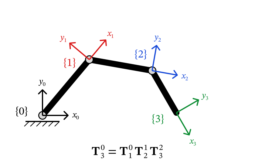
Figure 4.1 — One frame per link. Chaining the one-step postures gives the last frame relative to the ground.
The widget below shows frames , , on the 2R arm from Chapter 3, placed as in the lecture notes: frame at the elbow with along link 1, and frame at the tip with along link 2. Move the sliders: frame only reacts to , while frame is carried by both joints.
def rot2(theta):
    # 2x2 rotation matrix for an angle theta (radians), counter-clockwise.
    c, s = np.cos(theta), np.sin(theta)
    return np.array([[c, -s],
                     [s,  c]])


def draw_frame_2d(ax, R, origin, name='', scale=0.25):
    # Draw a 2D frame: column 1 of R is the x axis (red), column 2 the y axis (green).
    o = np.asarray(origin, float)
    for i, (col, lbl) in enumerate(zip(AXIS_COLORS[:2], 'xy')):
        v = R[:, i] * scale
        ax.annotate('', xy=o + v, xytext=o,
                    arrowprops=dict(arrowstyle='->', color=col, lw=2))
        ax.text(*(o + v * 1.35), f'${lbl}_{{{name}}}$' if name else lbl,
                color=col, fontsize=10, fontweight='bold')
    if name:
        ax.text(o[0] - 0.16, o[1] - 0.16, '{' + name + '}', fontsize=11, fontweight='bold')


def frames_on_2R_demo(theta1_deg, theta2_deg):
    L1, L2 = 1.0, 0.8
    t1, t2 = np.radians(theta1_deg), np.radians(theta2_deg)

    # frame {1} at the elbow (x1 along link 1), frame {2} at the tip (x2 along link 2)
    R10, o10 = rot2(t1),      np.array([L1*np.cos(t1), L1*np.sin(t1)])
    R20, o20 = rot2(t1 + t2), o10 + np.array([L2*np.cos(t1+t2), L2*np.sin(t1+t2)])

    fig, ax = plt.subplots(figsize=(6, 6))
    ax.plot([0, o10[0]], [0, o10[1]], color='steelblue', lw=6, solid_capstyle='round')
    ax.plot([o10[0], o20[0]], [o10[1], o20[1]], color='tomato', lw=6, solid_capstyle='round')
    draw_frame_2d(ax, np.eye(2), [0, 0], '0')
    draw_frame_2d(ax, R10, o10, '1')
    draw_frame_2d(ax, R20, o20, '2')

    r = L1 + L2 + 0.3
    ax.set_xlim(-r, r); ax.set_ylim(-r, r)
    ax.set_aspect('equal'); ax.grid(True, alpha=0.3)
    ax.set_title('Each link carries its own frame', fontsize=11)
    ax.set_xlabel('$x_0$'); ax.set_ylabel('$y_0$')
    plt.tight_layout(); plt.show()


interact(frames_on_2R_demo,
         theta1_deg=FloatSlider(value=45, min=-180, max=180, step=1, description='θ₁ (°)'),
theta2_deg=FloatSlider(value=60, min=-180, max=180, step=1, description='θ₂ (°)'));Key Takeaways — Section 4.1
A coordinate frame = an origin + perpendicular unit axes.
Attach one frame to each link; the frame moves with its link.
Describe each frame relative to the one before it, , then chain: .
4.2 Posture in 2D
The posture of frame relative to frame has two parts:
position — where is the origin ?
orientation — which way do the axes point?
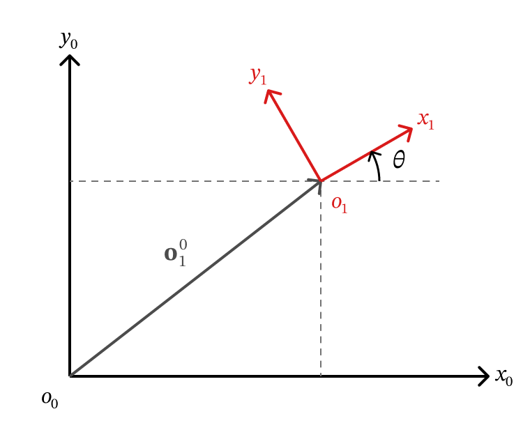
Figure 4.2 — Posture of frame {1} relative to frame {0}: position o10 and orientation θ.
4.2.1 Position
The position is the vector from to , written in frame :
(Seen from frame itself, its own origin is always . The superscript matters!)
4.2.2 Orientation: the 2D rotation matrix
Frame is turned counter-clockwise by relative to frame . We record its orientation by writing its own axes in frame , side by side:
From the drawing, the unit vector has a component along and along ; the unit vector has along and along . So
Another way to get the entries — dot products. Recall the inner (dot) product . If is a unit vector, is simply the length of the shadow of on , i.e. the component of along . So every entry of the rotation matrix is “how much of one axis lies along another”:
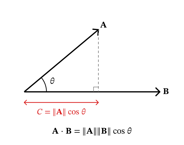
Figure 4.3 — The dot product with a unit vector is the length of the shadow (projection).
Column 1 is seen from frame , column 2 is seen from frame . Move the slider and watch the printed columns follow the red and green arrows.
def rotation_demo(theta_deg):
    theta = np.radians(theta_deg)
    R10 = rot2(theta)
    shape = np.array([[0, 0], [1, 0], [1, .2], [.2, .2], [.2, 1], [0, 1], [0, 0]]).T   # an "L" shape

    fig, axes = plt.subplots(1, 2, figsize=(11, 5))
    for ax, R, title in zip(axes, [np.eye(2), R10],
                            ['Frame {0}', f'Frame {{1}}, turned by θ = {theta_deg:.0f}°']):
        pts = R @ shape
        ax.fill(pts[0], pts[1], alpha=0.3, color='steelblue')
        ax.plot(pts[0], pts[1], color='steelblue', lw=2)
        for vec, col, lbl in [(R[:, 0], 'red', 'x'), (R[:, 1], 'green', 'y')]:
            ax.annotate('', xy=0.5*vec, xytext=[0, 0],
                        arrowprops=dict(arrowstyle='->', color=col, lw=2.5))
            ax.text(*(0.6*vec), lbl, color=col, fontsize=13, fontweight='bold')
        ax.set_xlim(-1.5, 1.5); ax.set_ylim(-1.5, 1.5)
        ax.set_aspect('equal'); ax.grid(True, alpha=0.3)
        ax.set_title(title, fontsize=12)
        ax.set_xlabel('$x_0$'); ax.set_ylabel('$y_0$')

    print(f'R_1^0 =\n{R10}')
    print(f'\ncolumn 1 = x_1 in frame 0: {R10[:, 0]}')
    print(f'column 2 = y_1 in frame 0: {R10[:, 1]}')
    plt.tight_layout(); plt.show()


interact(rotation_demo,
theta_deg=FloatSlider(value=30, min=-180, max=180, step=5, description='θ (°)'));4.2.3 A rotation matrix converts coordinates between frames
Here is the main job of a rotation matrix (Lecture 6). Frames and share an origin; points along and points along (frame is turned by ).
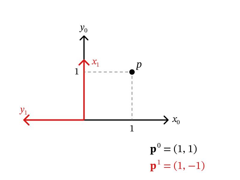
Figure 4.4 — Lecture 6 example: the same point p described in frame {0} and in frame {1}.
Read the columns off the drawing:
A point sits at 1 along and 1 along , so . Measured along frame 's axes it is 1 along and -1 along , so . The rotation matrix connects the two:
Going the other way. Swap the roles of the frames: holds frame 's axes seen from frame . From the drawing, points along and along :
So to go back, just transpose — no matrix inversion needed.
Why is the inverse just the transpose? (click to expand)
The entries of \mathbf{R}_1^0 are dot products: row i, column j is (axis j of frame 1)\cdot(axis i of frame 0). For \mathbf{R}_0^1 the roles swap, which swaps rows and columns — a transpose. Since going 0\to1\to0 must change nothing, \mathbf{R}_0^1\mathbf{R}_1^0 = \mathbf{I}, i.e. (\mathbf{R}_1^0)^{-1} = (\mathbf{R}_1^0)^\top.
Three properties every rotation matrix has:
| Property | In plain words |
|---|---|
| the columns are unit vectors at right angles to each other | |
| going back is a transpose | |
| it only turns things — no stretching and no mirror image |
# Lecture 6 example: x1 along y0, y1 along -x0
R10 = np.array([[0, -1],
                [1,  0]])          # columns: x_1^0, y_1^0
p1  = np.array([1, -1])            # p in frame {1}

p0 = R10 @ p1
print('p^0 = R_1^0 p^1      =', p0)

R01 = R10.T                        # R_0^1 = (R_1^0)^T
print('R_0^1 =\n', R01)
print('p^1 = R_0^1 p^0      =', R01 @ p0)

print('\nR^T R = I ?', np.allclose(R10.T @ R10, np.eye(2)),
      '    det(R) =', round(np.linalg.det(R10), 6))
print('R_1^0 equals rot2(90°)?', np.allclose(R10, rot2(np.radians(90))))
p^0 = R_1^0 p^1 = [1 1]
R_0^1 =
[[ 0 1]
[-1 0]]
p^1 = R_0^1 p^0 = [ 1 -1]
R^T R = I ? True det(R) = 1.0
R_1^0 equals rot2(90°)? True
4.2.4 Combining two rotations in 2D
If frame is turned by relative to frame , and frame is turned by relative to frame , the indices chain just like in Section 4.1:
In 2D the angles simply add, so the order does not matter: . For the 2R arm this is the familiar fact that link 2 points at the angle .
Careful: this “order does not matter” is special to 2D. In 3D the order of rotations does matter (Section 4.3.2).
def composition_2d_demo(alpha_deg, beta_deg):
    Ra, Rb = rot2(np.radians(alpha_deg)), rot2(np.radians(beta_deg))
    shape = np.array([[0, 0], [1, 0], [1, .2], [.2, .2], [.2, 1], [0, 1], [0, 0]]).T

    fig, axes = plt.subplots(1, 3, figsize=(15, 5))
    for ax, (R, ttl) in zip(axes, [(np.eye(2), 'Frame {0}'),
                                   (Ra @ Rb, f'R({alpha_deg:.0f}°) R({beta_deg:.0f}°)'),
                                   (Rb @ Ra, f'R({beta_deg:.0f}°) R({alpha_deg:.0f}°)')]):
        pts = R @ shape
        ax.fill(pts[0], pts[1], alpha=0.3, color='steelblue')
        ax.plot(pts[0], pts[1], 'steelblue', lw=2)
        for vec, col in [(R[:, 0], 'red'), (R[:, 1], 'green')]:
            ax.annotate('', xy=0.45*vec, xytext=[0, 0],
                        arrowprops=dict(arrowstyle='->', color=col, lw=2.5))
        ax.set_xlim(-1.6, 1.6); ax.set_ylim(-1.6, 1.6)
        ax.set_aspect('equal'); ax.grid(True, alpha=0.3)
        ax.set_title(ttl, fontsize=11)

    print('R(α)R(β) = R(α+β)?            ', np.allclose(Ra @ Rb, rot2(np.radians(alpha_deg + beta_deg))))
    print('R(α)R(β) = R(β)R(α)?  (2D only)', np.allclose(Ra @ Rb, Rb @ Ra))
    plt.tight_layout(); plt.show()


interact(composition_2d_demo,
         alpha_deg=FloatSlider(value=45, min=-180, max=180, step=5, description='α (°)'),
beta_deg =FloatSlider(value=30, min=-180, max=180, step=5, description='β (°)'));4.2.5 Position + orientation together: the 2D HTM
Now frame is both moved (origin at ) and turned (). A point has coordinates in frame . Where is it in frame ? Think of it as two moves (Lecture 6):
Turn the arrow from to into frame- directions: .
Add where that arrow starts, : .
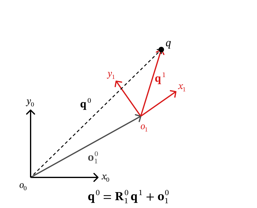
Figure 4.5 — A point q seen from a moved and turned frame: q0 = R10 q1 + o10.
That’s correct, but it is a multiply and an add. With many frames in a chain we’d alternate multiply, add, multiply, add… There’s a neat trick to fold both into one multiplication: put a 1 under each point and pack and into one bigger matrix:
Multiply the first two rows out and you get exactly ; the third row just says . The extra row and column are bookkeeping, not new physics. is the homogeneous transformation matrix: the posture (position and orientation) of frame relative to frame .
Worked example. Frame has its origin at and is turned by ( along , along ). A point is 1 unit along : . Then
Sanity check with a sketch: start at and walk 1 unit along , which points “up” (). You land at . ✓
def htm_2d(theta, o):
    # 3x3 HTM T_1^0 from the angle theta of frame {1} and its origin o = o_1^0.
    T = np.eye(3)
    T[:2, :2] = rot2(theta)
    T[:2,  2] = o
    return T


# Worked example: o_1^0 = (1, 1), frame {1} turned by 90°, q^1 = (1, 0)
T10 = htm_2d(np.radians(90), [1, 1])
q1  = np.array([1, 0])

q0_two_steps = T10[:2, :2] @ q1 + T10[:2, 2]     # R_1^0 q^1 + o_1^0
q0_tilde     = T10 @ np.append(q1, 1)            # T_1^0 [q^1; 1]

print('T_1^0 =\n', T10)
print('\nR q1 + o          :', q0_two_steps)
print('T_1^0 [q1; 1]     :', q0_tilde, ' -> q^0 =', q0_tilde[:2])

T01 = np.linalg.inv(T10)                         # T_0^1 = (T_1^0)^-1  (Section 4.4.3 shows a shortcut)
print('\nBack again, T_0^1 [q0; 1] :', T01 @ q0_tilde, ' -> q^1 =', (T01 @ q0_tilde)[:2])
T_1^0 =
[[ 0. -1. 1.]
[ 1. 0. 1.]
[ 0. 0. 1.]]
R q1 + o : [1. 2.]
T_1^0 [q1; 1] : [1. 2. 1.] -> q^0 = [1. 2.]
Back again, T_0^1 [q0; 1] : [1. 0. 1.] -> q^1 = [1. 0.]
4.2.6 Example: forward kinematics of the 2R arm with HTMs
Let’s redo the Chapter 3 problem with HTMs (Lecture 6). Frames as in the widget of Section 4.1: frame at the elbow with along link 1, frame at the tip with along link 2. Shorthand: , , and so on.
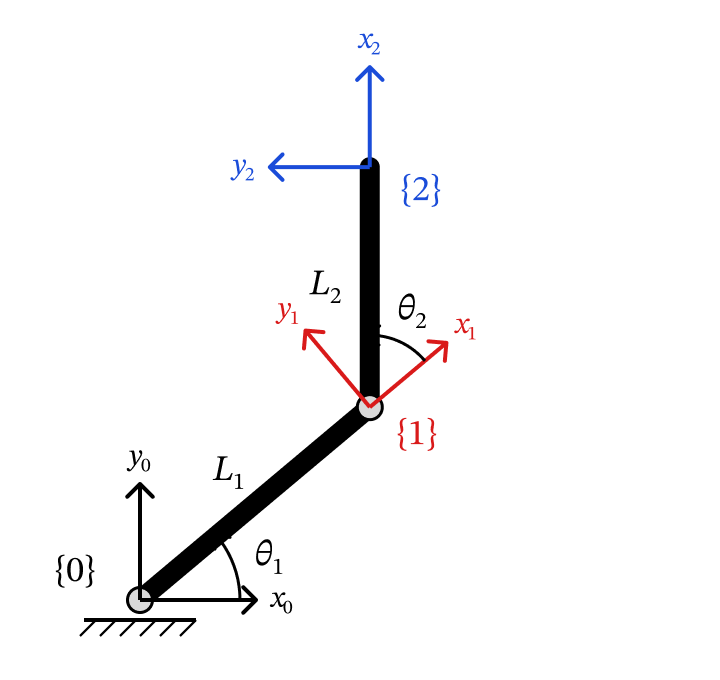
Figure 4.6 — The 2R arm with frame {1} at the elbow and frame {2} at the tip (as in the lecture notes).
Step 1 — frame relative to frame . is turned by , and is at the end of link 1:
Step 2 — frame relative to frame . Seen from frame , link 2 is turned by and has length — exactly the same form:
Step 3 — chain them. The tip is the origin . In its own frame it is , so
Using and :
— exactly the Chapter 3 answer, but now produced by a recipe (write one HTM per link, multiply) instead of by staring at triangles. The product also gives the tip’s orientation for free: its rotation block is .
Chapter 5 places the frames slightly differently (frame sits on joint , with along the joint axis, and an extra frame at the gripper). That choice makes the recipe work for any 3D robot. The tip position comes out the same.
The cell below lets SymPy do the algebra of Step 3 for us.
t1, t2, L1s, L2s = sp.symbols('theta_1 theta_2 L_1 L_2', real=True)

def sym_htm_2d(theta, L):
    # Symbolic T_i^{i-1} for a planar link: turned by theta, origin at the end of a link of length L.
    c, s = sp.cos(theta), sp.sin(theta)
    return sp.Matrix([[c, -s, L*c],
                      [s,  c, L*s],
                      [0,  0, 1]])

T10_s = sym_htm_2d(t1, L1s)
T21_s = sym_htm_2d(t2, L2s)
T20_s = sp.simplify(T10_s * T21_s)            # T_2^0 = T_1^0 T_2^1

display(Math(r'\mathbf{T}_2^0 = \mathbf{T}_1^0\,\mathbf{T}_2^1 = ' + sp.latex(T20_s)))
display(Math(r'\tilde{\mathbf{o}}_2^0 = \mathbf{T}_2^0\,[0,\ 0,\ 1]^\top = '
+ sp.latex(sp.simplify(T20_s * sp.Matrix([0, 0, 1])))))def fk_ch3(theta1, theta2, L1=1.0, L2=0.8):
# The Chapter 3 trig formula, used as the answer to check against.
return np.array([L1*np.cos(theta1) + L2*np.cos(theta1 + theta2),
L1*np.sin(theta1) + L2*np.sin(theta1 + theta2)])
def htm_chain_demo(theta1_deg, theta2_deg):
L1, L2 = 1.0, 0.8
t1, t2 = np.radians(theta1_deg), np.radians(theta2_deg)
T10 = htm_2d(t1, [L1*np.cos(t1), L1*np.sin(t1)]) # frame {1} relative to frame {0}
T21 = htm_2d(t2, [L2*np.cos(t2), L2*np.sin(t2)]) # frame {2} relative to frame {1}
T20 = T10 @ T21 # chain: frame {2} relative to frame {0}
o10, o20 = T10[:2, 2], T20[:2, 2]
fig, ax = plt.subplots(figsize=(6, 6))
ax.plot([0, o10[0]], [0, o10[1]], color='steelblue', lw=6, solid_capstyle='round')
ax.plot([o10[0], o20[0]], [o10[1], o20[1]], color='tomato', lw=6, solid_capstyle='round')
draw_frame_2d(ax, np.eye(2), [0, 0], '0')
draw_frame_2d(ax, T10[:2, :2], o10, '1')
draw_frame_2d(ax, T20[:2, :2], o20, '2')
ax.plot(*o20, 'g*', markersize=15, zorder=5)
r = L1 + L2 + 0.3
ax.set_xlim(-r, r); ax.set_ylim(-r, r)
ax.set_aspect('equal'); ax.grid(True, alpha=0.3)
ax.set_title(f'Tip from the HTM chain: ({o20[0]:.3f}, {o20[1]:.3f})', fontsize=11)
ax.set_xlabel('$x_0$'); ax.set_ylabel('$y_0$')
plt.tight_layout(); plt.show()
print('Tip from T_1^0 T_2^1 :', o20)
print('Tip from the Chapter 3 formula:', fk_ch3(t1, t2, L1, L2))
print('Match?', np.allclose(o20, fk_ch3(t1, t2, L1, L2)))
interact(htm_chain_demo,
theta1_deg=FloatSlider(value=45, min=-180, max=180, step=1, description='θ₁ (°)'),
theta2_deg=FloatSlider(value=60, min=-180, max=180, step=1, description='θ₂ (°)'));Key Takeaways — Section 4.2
Posture = position + orientation .
: the columns are frame 's axes written in frame . Each entry is a dot product of two axes.
A rotation matrix converts coordinates: ; to go back, transpose: .
Moved and turned frame: , or in one step with .
Chaining frames is matrix multiplication: . For the 2R arm this reproduces Chapter 3’s formula.
4.3 Orientation in 3D
4.3.1 The 3D rotation matrix
Everything from 2D carries over — we just add the axis (Lecture 7). The orientation of frame relative to frame is again “frame 1’s axes, written in frame 0”:
For simple drawings where every axis of frame lines up with some axis of frame , each column is just one and two zeros: ask “which way does point, in frame-0 terms?”
Example 1. points along , points along , points along :
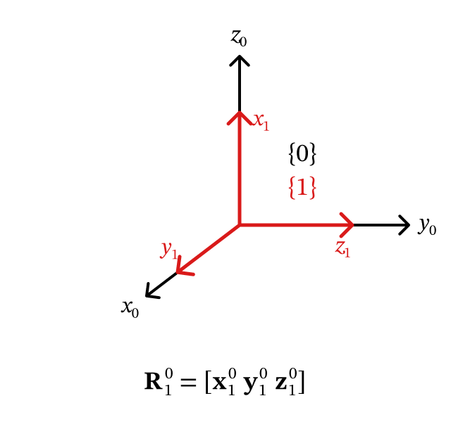
Figure 4.7 — Example 1: every axis of frame {1} lines up with an axis of frame {0}.
Example 2 (tilted axes). , , and all lie in one plane; is from , and points along . Use the dot products — for unit vectors :
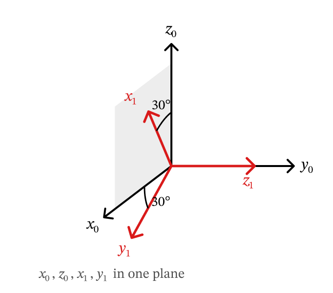
Figure 4.8 — Example 2: x1 is tilted 30° from z0; z1 points along y0.
Right-hand rule check. In a right-handed frame . You can use this to fill in a column you can’t see in the drawing, or to catch a mistake: if (equivalently ), something is wrong.
def draw_frame_3d(ax, R=None, origin=None, name='', scale=0.4, alpha=1.0):
    # Draw a 3D frame: columns of R are the x (red), y (green), z (blue) axes.
    R = np.eye(3) if R is None else R
    o = np.zeros(3) if origin is None else np.asarray(origin, float)
    for i, (col, lbl) in enumerate(zip(AXIS_COLORS, 'xyz')):
        v = R[:, i] * scale
        ax.quiver(*o, *v, color=col, alpha=alpha, arrow_length_ratio=0.2,
                  linewidth=max(0.5, 2*alpha))
        if alpha >= 0.5:
            ax.text(*(o + v*1.3), f'${lbl}_{{{name}}}$' if name else lbl,
                    color=col, fontsize=10, fontweight='bold', alpha=alpha)


def setup_3d(ax, lim=1.2, title=''):
    ax.set_xlim(-lim, lim); ax.set_ylim(-lim, lim); ax.set_zlim(-lim, lim)
    ax.set_xlabel('$x_0$'); ax.set_ylabel('$y_0$'); ax.set_zlabel('$z_0$')
    ax.set_title(title, fontsize=11)


c30, s30 = np.cos(np.radians(30)), np.sin(np.radians(30))
R10_ex1 = np.array([[0, 1, 0],
                    [0, 0, 1],
                    [1, 0, 0]], float)
R10_ex2 = np.array([[s30,  c30, 0],
                    [0,    0,   1],
                    [c30, -s30, 0]])

fig = plt.figure(figsize=(12, 5))
for k, (R, ttl) in enumerate([(R10_ex1, 'Example 1'), (R10_ex2, 'Example 2')]):
    ax = fig.add_subplot(1, 2, k + 1, projection='3d')
    draw_frame_3d(ax, np.eye(3), name='0', scale=0.9, alpha=0.6)
    draw_frame_3d(ax, R, name='1', scale=0.6)
    setup_3d(ax, 1.0, ttl)
    ax.view_init(20, 30)
plt.tight_layout(); plt.show()

for name, R in [('Example 1', R10_ex1), ('Example 2', R10_ex2)]:
    print(f'{name}:  x1 × y1 = z1 ? {np.allclose(np.cross(R[:, 0], R[:, 1]), R[:, 2])}'
          f'   det = {np.linalg.det(R):.3f}   R^T R = I ? {np.allclose(R.T @ R, np.eye(3))}')
print('\nExample 1:  R_0^1 = (R_1^0)^T =\n', R10_ex1.T)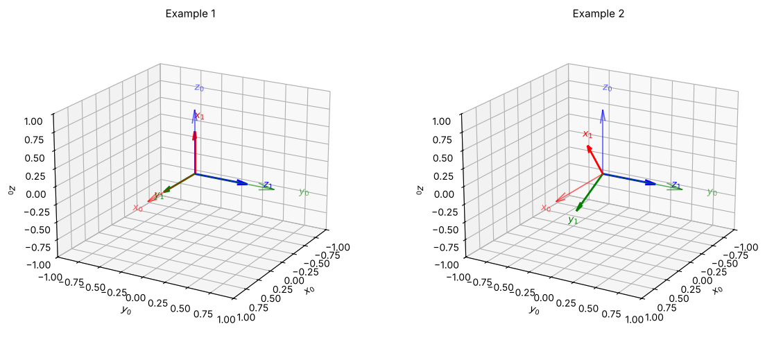
Example 1:  x1 × y1 = z1 ? True   det = 1.000   R^T R = I ? True
Example 2:  x1 × y1 = z1 ? True   det = 1.000   R^T R = I ? True

Example 1:  R_0^1 = (R_1^0)^T =
 [[0. 0. 1.]
 [1. 0. 0.]
 [0. 1. 0.]]
Converting coordinates in 3D
Exactly as in 2D:
Example (Lecture 7). Use the frames of Example 1. A point lies in the plane, 1 unit along and 1 unit along , so . Measured along frame 's axes it is 1 along (which points along ) and 1 along (which points along ), so . Check:
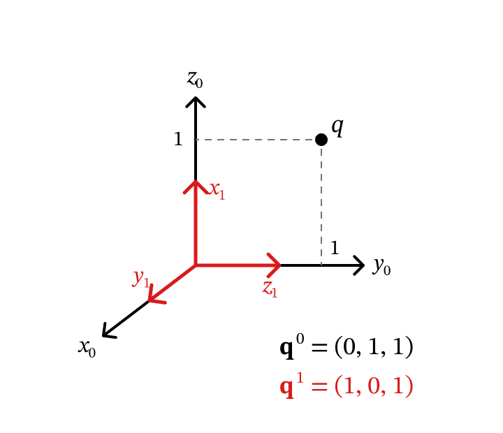
Figure 4.9 — Lecture 7 example: point q in the y0z0 plane, using the frames of Example 1.
q1 = np.array([1, 0, 1])
q0 = R10_ex1 @ q1
print('q^0 = R_1^0 q^1 =', q0)
print('q^1 = R_0^1 q^0 =', R10_ex1.T @ q0, '  (back where we started)')
q^0 = R_1^0 q^1 = [0. 1. 1.]
q^1 = R_0^1 q^0 = [1. 0. 1.] (back where we started)
The three basic rotation matrices
A rotation matrix can also describe a motion: start with frame on top of frame , then turn it by about one of frame 's axes. Reading the new axes column by column gives three special cases (Lecture 7):
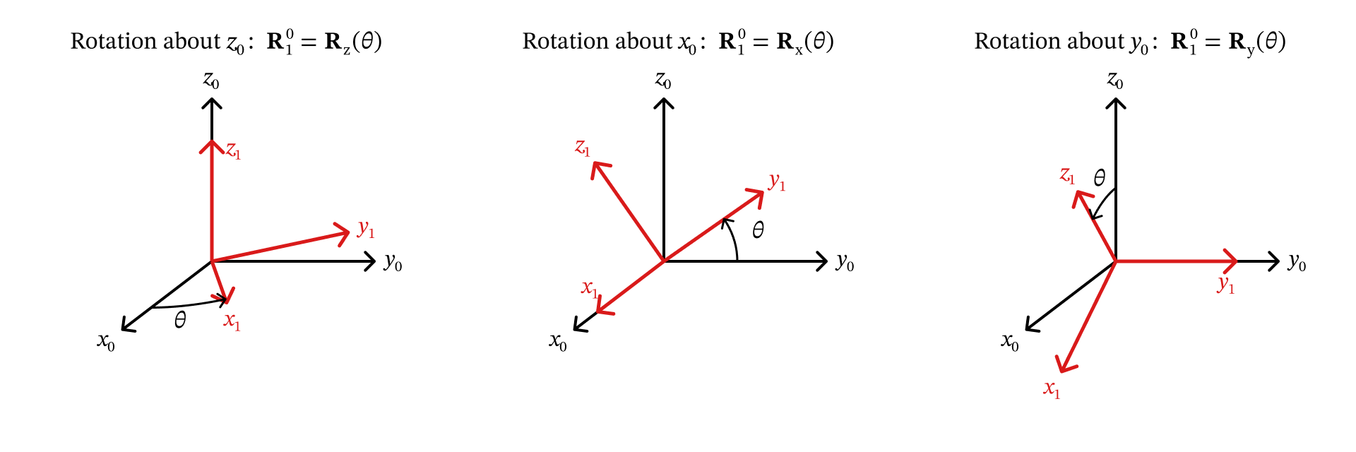
Figure 4.10 — The three basic rotations: frame {1} turned by θ about z0, x0, or y0.
Ways to remember them:
The axis you rotate about doesn’t move, so its row and column are a 1 and zeros.
The other block is the 2D rotation matrix.
looks “flipped” (the minus sign is at the bottom left). That is not a typo: about , the right-hand rule turns toward (the order is , not ), so a positive tips toward .
In Chapter 5 these become the rotation blocks of the basic HTMs , , .
def Rx(theta):
    c, s = np.cos(theta), np.sin(theta)
    return np.array([[1, 0,  0],
                     [0, c, -s],
                     [0, s,  c]])

def Ry(theta):
    c, s = np.cos(theta), np.sin(theta)
    return np.array([[ c, 0, s],
                     [ 0, 1, 0],
                     [-s, 0, c]])

def Rz(theta):
    c, s = np.cos(theta), np.sin(theta)
    return np.array([[c, -s, 0],
                     [s,  c, 0],
                     [0,  0, 1]])


def basic_rotation_demo(axis, angle_deg):
    theta = np.radians(angle_deg)
    R10 = {'about x₀': Rx, 'about y₀': Ry, 'about z₀': Rz}[axis](theta)

    fig = plt.figure(figsize=(11, 5))
    ax = fig.add_subplot(1, 2, 1, projection='3d')
    draw_frame_3d(ax, np.eye(3), scale=0.9, alpha=0.2)
    draw_frame_3d(ax, R10, name='1', scale=0.7)
    t, r = np.linspace(0, theta, 60), 0.55          # dashed arc showing the turn
    arc = {'about x₀': [0*t, r*np.cos(t), r*np.sin(t)],
           'about y₀': [r*np.sin(t), 0*t, r*np.cos(t)],
           'about z₀': [r*np.cos(t), r*np.sin(t), 0*t]}[axis]
    ax.plot(*arc, 'k--', lw=1.5, alpha=0.6)
    setup_3d(ax, 1.0, f'Rotate {axis} by θ = {angle_deg}°')

    ax2 = fig.add_subplot(1, 2, 2); ax2.axis('off')
    rows = '\n'.join('  '.join(f'{v:7.3f}' for v in row) for row in R10)
    ax2.text(0.05, 0.6, f'R_1^0 =\n\n{rows}\n\n   x_1^0    y_1^0    z_1^0', fontsize=13,
             fontfamily='monospace', va='center', transform=ax2.transAxes,
             bbox=dict(boxstyle='round', facecolor='lightyellow', alpha=0.6))
    ax2.text(0.05, 0.12, f'det = {np.linalg.det(R10):.4f}    R^T R = I ? {np.allclose(R10.T @ R10, np.eye(3))}',
             fontsize=11, fontfamily='monospace', transform=ax2.transAxes)
    plt.tight_layout(); plt.show()


interact(basic_rotation_demo,
         axis=ToggleButtons(options=['about z₀', 'about x₀', 'about y₀'], description='Axis'),
angle_deg=FloatSlider(value=45, min=-180, max=180, step=5, description='θ (°)'));4.3.2 Combining Rotations: Order Matters, and Fixed vs. Current Axes
In 3D, order matters. Take a book. Turn it about , then about . Now start again and do first, then . The book ends up in two different poses. So unlike 2D, we can’t just add up angles; we have to multiply matrices in the right order.
R_A = Ry(np.pi/2) @ Rx(np.pi/2)
R_B = Rx(np.pi/2) @ Ry(np.pi/2)

fig = plt.figure(figsize=(12, 5))
fig.suptitle('Same two 90° turns, different order', fontsize=13, fontweight='bold')
for i, (R, ttl) in enumerate([(R_A, 'R_y(90°) R_x(90°)'), (R_B, 'R_x(90°) R_y(90°)')]):
    ax = fig.add_subplot(1, 2, i + 1, projection='3d')
    draw_frame_3d(ax, np.eye(3), alpha=0.15, scale=0.9)
    draw_frame_3d(ax, R, name='1', scale=0.7)
    setup_3d(ax, 1.0, ttl)
plt.tight_layout(); plt.show()

print('R_y(90°) R_x(90°) =\n', R_A)
print('\nR_x(90°) R_y(90°) =\n', R_B)
print('\nEqual?', np.allclose(R_A, R_B), ' <- in 3D, order matters!')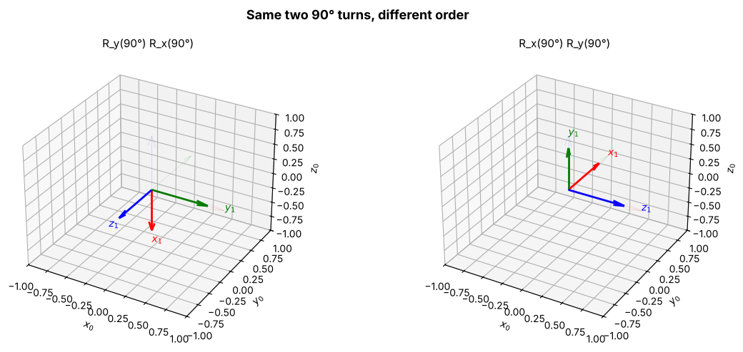
R_y(90°) R_x(90°) =
 [[ 0.  1.  0.]
 [ 0.  0. -1.]
 [-1.  0.  0.]]

R_x(90°) R_y(90°) =
 [[ 0.  0.  1.]
 [ 1.  0. -0.]
 [-0.  1.  0.]]

Equal? False  <- in 3D, order matters!
Which axis does a new rotation act about? It depends on which side you multiply on.
| You write | The new rotation turns the frame about … | Name |
|---|---|---|
| the frame’s current (own, “body”) axes | post-multiply (on the right) | |
| the fixed axes of frame | pre-multiply (on the left) |
Why the right side means “current axes”. Write it with frames: . The extra rotation describes frame relative to frame — so it is measured about frame 's own axes, wherever they currently point. This is the rule we use all the time in Chapter 5: a product like is read left to right, each turn about the frame’s current axes.
Picture it: a drone. “Pitch up relative to where my nose points” (what the pilot does) is post-multiplication. “Tilt about the room’s fixed axis, whichever way I’m facing” is pre-multiplication.
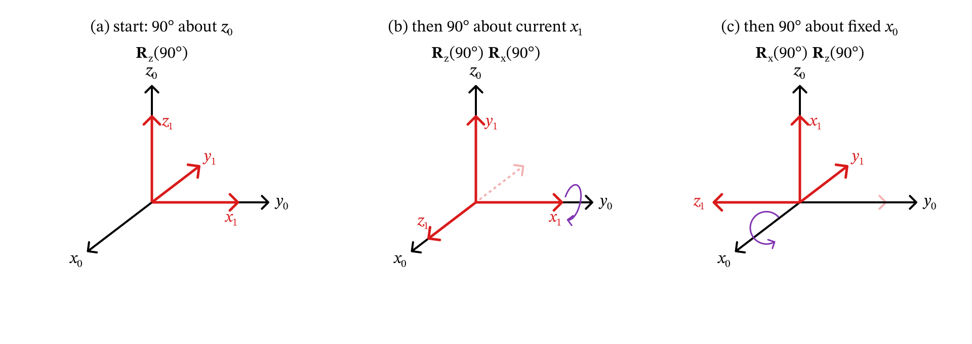
Figure 4.11 — Same second turn, different axis: about the current x1 (multiply on the right) vs. the fixed x0 (multiply on the left).
The widget starts from the pose and adds on either side. Watch which blue axis the frame spins about: its own (bold), or the faded fixed .
def prepost_demo(angle_deg, order):
    R_cur = Ry(np.radians(45)) @ Rx(np.radians(30))     # starting pose
    R_add = Rz(np.radians(angle_deg))
    if order == 'R_current · R_z(θ)  → current axis':
        R_new = R_cur @ R_add
    else:
        R_new = R_add @ R_cur

    fig = plt.figure(figsize=(12, 5))
    for i, (R, ttl) in enumerate([(R_cur, 'Start: R_y(45°) R_x(30°)'),
                                  (R_new, order.split('→')[0] + f' with θ = {angle_deg}°')]):
        ax = fig.add_subplot(1, 2, i + 1, projection='3d')
        draw_frame_3d(ax, np.eye(3), scale=1.0, alpha=0.2)
        draw_frame_3d(ax, R_cur, scale=0.7, alpha=0.25)          # ghost of the starting pose
        draw_frame_3d(ax, R, name='1', scale=0.7)
        setup_3d(ax, 1.1, ttl)
    plt.tight_layout(); plt.show()


interact(prepost_demo,
         angle_deg=FloatSlider(value=60, min=-180, max=180, step=5, description='θ (°)'),
         order=ToggleButtons(options=['R_current · R_z(θ)  → current axis',
                                      'R_z(θ) · R_current  → fixed axis'],
description='Order', style={'button_width': '260px'}));4.3.3 Other Ways to Describe 3D Orientation
A rotation matrix has 9 numbers, but only 3 of them are independent — an orientation has 3 degrees of freedom (think yaw, pitch, roll). Robotics software uses several other, more compact descriptions. You will meet all of them in libraries like MuJoCo, ROS and SciPy:
| Representation | # numbers | Good for | Watch out for |
|---|---|---|---|
| Rotation matrix | 9 | computing, chaining frames | 6 of the 9 numbers are redundant |
| Axis-angle | 4 (axis + angle) | intuition: “one spin about one axis” | the axis is undefined when the angle is 0 |
| Euler angles | 3 | humans: yaw / pitch / roll | gimbal lock; 12 different conventions |
| Quaternion | 4 | smooth interpolation, simulators | less intuitive |
Rule of thumb: compute with rotation matrices, show Euler angles to humans, let the software use quaternions.
Axis-angle and Rodrigues’ formula
Idea: any 3D orientation can be reached with a single turn by some angle about some unit axis — like turning a screwdriver whose shaft points along . Rodrigues’ formula turns into a rotation matrix:
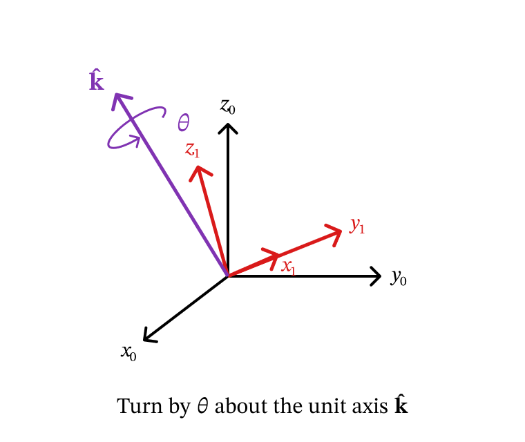
Figure 4.12 — Axis-angle: one turn by θ about a unit axis k̂.
is just the cross product written as a matrix: . You don’t need to memorize the formula; the useful facts are:
gives (no turn).
gives exactly — the basic rotations are special cases (try it in the widget: set ).
Libraries such as MuJoCo and ROS use this formula internally.
def skew(k):
    # [k]_x : the matrix with [k]_x @ v == np.cross(k, v)
    return np.array([[    0, -k[2],  k[1]],
                     [ k[2],     0, -k[0]],
                     [-k[1],  k[0],     0]])

def rodrigues(k_vec, theta):
    k = np.asarray(k_vec, float)
    k = k / np.linalg.norm(k)
    K = skew(k)
    return np.eye(3) + np.sin(theta)*K + (1 - np.cos(theta))*(K @ K)


print('Rodrigues with k = z-axis equals R_z(θ)?',
      np.allclose(rodrigues([0, 0, 1], 0.7), Rz(0.7)))


def axis_angle_demo(kx, ky, kz, angle_deg):
    k_raw = np.array([kx, ky, kz], float)
    if np.linalg.norm(k_raw) < 1e-6:
        print('The axis is the zero vector — make at least one component non-zero.'); return
    k = k_raw / np.linalg.norm(k_raw)
    R = rodrigues(k, np.radians(angle_deg))

    fig = plt.figure(figsize=(11, 5))
    ax = fig.add_subplot(1, 2, 1, projection='3d')
    draw_frame_3d(ax, np.eye(3), scale=0.9, alpha=0.15)
    draw_frame_3d(ax, R, name='1', scale=0.7)
    ax.quiver(0, 0, 0, *k*0.9, color='black', lw=2.5, arrow_length_ratio=0.15)
    ax.text(*k*1.05, 'k̂', fontsize=13, fontweight='bold')
    setup_3d(ax, 1.0, f'Turn {angle_deg}° about k̂ = [{k[0]:.2f}, {k[1]:.2f}, {k[2]:.2f}]')

    ax2 = fig.add_subplot(1, 2, 2); ax2.axis('off')
    rows = '\n'.join('  '.join(f'{v:7.3f}' for v in row) for row in R)
    ax2.text(0.05, 0.55, f'R (Rodrigues) =\n\n{rows}', fontsize=12, fontfamily='monospace',
             va='center', transform=ax2.transAxes,
             bbox=dict(boxstyle='round', facecolor='lightyellow', alpha=0.6))
    plt.tight_layout(); plt.show()


interact(axis_angle_demo,
         kx=FloatSlider(value=1.0, min=-1, max=1, step=0.1, description='k_x'),
         ky=FloatSlider(value=1.0, min=-1, max=1, step=0.1, description='k_y'),
         kz=FloatSlider(value=1.0, min=-1, max=1, step=0.1, description='k_z'),
         angle_deg=FloatSlider(value=120, min=-180, max=180, step=5, description='θ (°)'));
Rodrigues with k = z-axis equals R_z(θ)? True
Euler angles — ZYX (yaw, pitch, roll)
Euler angles build an orientation from three turns in a row about coordinate axes. The most common convention in robotics and aviation is ZYX, also called yaw–pitch–roll:
| Angle | Axis | Name | Think of … |
|---|---|---|---|
| yaw | compass heading | ||
| pitch | nose up / down | ||
| roll | tilting the wings |
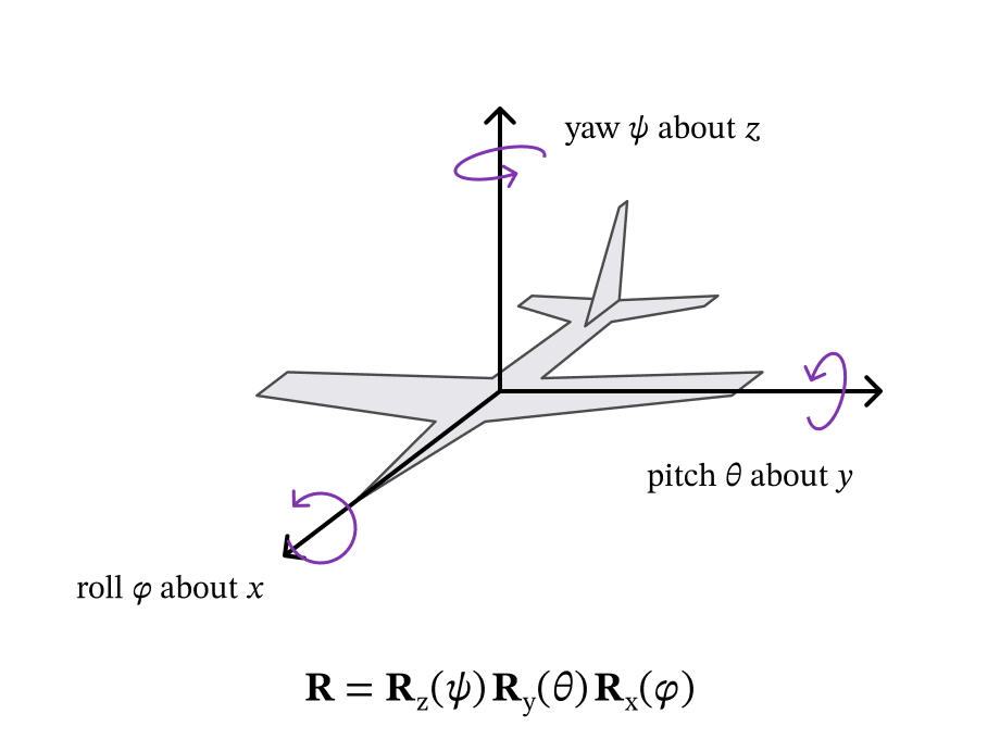
Figure 4.13 — Yaw ψ about z, pitch θ about y, roll φ about x.
Read the product left to right with the rule from Section 4.3.2: first yaw about , then pitch about the new , then roll about the newest — each turn about the current axes.
Gimbal lock. When the pitch is , the yaw axis and the roll axis line up, so yaw and roll do the same thing and one degree of freedom is lost. Try it in the widget: set pitch to and move yaw and roll — they produce the same kind of motion.
You’ll see another convention in Chapter 5: a spherical wrist produces , the ZYZ Euler angles.
def euler_zyx_demo(yaw_deg, pitch_deg, roll_deg):
    R = Rz(np.radians(yaw_deg)) @ Ry(np.radians(pitch_deg)) @ Rx(np.radians(roll_deg))
    near_lock = abs(pitch_deg) >= 85
    color = 'crimson' if near_lock else 'black'

    fig = plt.figure(figsize=(12, 5))
    ax = fig.add_subplot(1, 2, 1, projection='3d')
    draw_frame_3d(ax, np.eye(3), scale=0.9, alpha=0.15)
    draw_frame_3d(ax, R, name='1', scale=0.7)
    setup_3d(ax, 1.0, f'yaw ψ={yaw_deg}°, pitch θ={pitch_deg}°, roll φ={roll_deg}°'
                       + ('  ⚠ GIMBAL LOCK' if near_lock else ''))
    ax.title.set_color(color)

    ax2 = fig.add_subplot(1, 2, 2); ax2.axis('off')
    rows = '\n'.join('  '.join(f'{v:7.3f}' for v in row) for row in R)
    info = f'R = Rz({yaw_deg}°) Ry({pitch_deg}°) Rx({roll_deg}°)\n\n{rows}'
    if near_lock:
        info += '\n\nPitch ≈ ±90°: yaw and roll now\nturn about the same axis.'
    ax2.text(0.05, 0.55, info, fontsize=11, fontfamily='monospace', va='center',
             transform=ax2.transAxes, color=color,
             bbox=dict(boxstyle='round', facecolor='mistyrose' if near_lock else 'lightyellow',
                       alpha=0.6))
    plt.tight_layout(); plt.show()


interact(euler_zyx_demo,
         yaw_deg  =FloatSlider(value=30, min=-180, max=180, step=5, description='Yaw ψ (z)'),
         pitch_deg=FloatSlider(value=20, min=-90,  max=90,  step=5, description='Pitch θ (y)'),
roll_deg =FloatSlider(value=10, min=-180, max=180, step=5, description='Roll φ (x)'));Quaternions
A unit quaternion stores an orientation in four numbers: a scalar part and a 3-vector part . It is built straight from the axis-angle pair :
(We write quaternions as so they don’t get mixed up with points .) So a quaternion is really axis-angle, repackaged so that combining rotations becomes a simple multiplication.
Why bother?
No gimbal lock — every orientation is handled smoothly.
Smooth in-between orientations — SLERP turns at a constant rate from one orientation to another (great for animation and trajectories).
Cheap and numerically stable — that’s why simulators use them.
Watch the order of the four numbers. MuJoCo stores quaternions scalar-first,
— e.g. data.xquat, and qpos of free/ball joints. SciPy’s
Rotation uses scalar-last, . Mixing these up is one of the most
common bugs in robotics code.
In practice you let a library (scipy.spatial.transform.Rotation, or MuJoCo’s mju_*
functions) convert between representations. But it’s worth doing the two core
operations by hand once, so the library isn’t a black box.
Converting and combining quaternions by hand
1. Quaternion → rotation matrix. For :
2. Combining two rotations (the Hamilton product). The quaternion version of the matrix product is (same order):
It looks long, but it’s just a dot product for the scalar part and “weighted sum plus a cross product” for the vector part.
Bonus — the inverse is free (just like ): for a unit quaternion, flip the sign of the vector part, .
The cells below use exactly these formulas on numbers small enough to check on paper.
print('=== Quaternion from axis-angle: 90° about z ===\n')
k_hat = np.array([0.0, 0.0, 1.0])
theta = np.radians(90.0)

w = np.cos(theta / 2)
v = np.sin(theta / 2) * k_hat
print(f'Q = (cos45°, sin45°·k̂) = ({w:.4f}, {v[0]:.4f}, {v[1]:.4f}, {v[2]:.4f})')
print(f'|Q|² = {w**2 + v @ v:.6f}   (unit quaternion ✓)\n')

# --- The same thing with SciPy (scalar-LAST!) --------------------------------
r = Rotation.from_rotvec(theta * k_hat)
print('SciPy as_quat() (scalar-last)  :', r.as_quat().round(4))
print('reordered to (w, vx, vy, vz)    :', np.roll(r.as_quat(), 1).round(4))
print('\nSciPy rotation matrix equals R_z(90°)?', np.allclose(r.as_matrix(), Rz(np.pi/2)))

# --- SLERP: smooth in-between orientations ------------------------------------
print('\n=== SLERP from 0° to 90° about z ===')
r_start = Rotation.from_euler('z', 0, degrees=True)
r_end   = Rotation.from_euler('z', 90, degrees=True)
slerp = Slerp([0, 1], Rotation.concatenate([r_start, r_end]))
for t in [0.0, 0.25, 0.5, 0.75, 1.0]:
    print(f'  t = {t:.2f}  ->  angle about z = {slerp(t).as_euler("xyz", degrees=True)[2]:5.1f}°')
=== Quaternion from axis-angle: 90° about z ===
Q = (cos45°, sin45°·k̂) = (0.7071, 0.0000, 0.0000, 0.7071)
|Q|² = 1.000000 (unit quaternion ✓)
SciPy as_quat() (scalar-last) : [0. 0. 0.7071 0.7071]
reordered to (w, vx, vy, vz) : [0.7071 0. 0. 0.7071]
SciPy rotation matrix equals R_z(90°)? True
=== SLERP from 0° to 90° about z ===
t = 0.00 -> angle about z = 0.0°
t = 0.25 -> angle about z = 22.5°
t = 0.50 -> angle about z = 45.0°
t = 0.75 -> angle about z = 67.5°
t = 1.00 -> angle about z = 90.0°
Example 1 — Quaternions for the planar 2R arm
Every joint of the 2R arm turns about the same fixed axis, . So the orientation of each link frame is a single turn about and its quaternion is simply
Frame is turned by and frame by (Section 4.2.4). With , :
The cell below checks against using the
conversion formula, and — if mujoco is installed — against MuJoCo’s own data.xquat for
a 2R model like the one in Chapter 3. They agree up to an overall sign: and
describe the same orientation, so a library may return either.
def quat_to_matrix(Q):
    # Unit quaternion Q = (w, vx, vy, vz)  ->  3x3 rotation matrix.
    w, x, y, z = Q
    return np.array([
        [1 - 2*(y**2 + z**2), 2*(x*y - w*z),       2*(x*z + w*y)],
        [2*(x*y + w*z),       1 - 2*(x**2 + z**2), 2*(y*z - w*x)],
        [2*(x*z - w*y),       2*(y*z + w*x),       1 - 2*(x**2 + y**2)]])


def quat_mult(Qa, Qb):
    # Hamilton product Qa ⊗ Qb  (same order as the matrix product Ra @ Rb).
    wa, va = Qa[0], np.asarray(Qa[1:])
    wb, vb = Qb[0], np.asarray(Qb[1:])
    return np.array([wa*wb - va @ vb, *(wa*vb + wb*va + np.cross(va, vb))])


theta1, theta2 = np.radians(45), np.radians(60)
Q10 = np.array([np.cos(theta1/2), 0, 0, np.sin(theta1/2)])
Q20 = np.array([np.cos((theta1 + theta2)/2), 0, 0, np.sin((theta1 + theta2)/2)])
print('Q_1^0 =', Q10.round(4))
print('Q_2^0 =', Q20.round(4))
print('\nquat_to_matrix(Q_2^0) == R_z(θ1+θ2)?', np.allclose(quat_to_matrix(Q20), Rz(theta1 + theta2)))

# Optional cross-check with MuJoCo
try:
    import mujoco
    XML_2R = '''
    <mujoco>
      <worldbody>
        <body name="link1">
          <joint name="joint1" type="hinge" axis="0 0 1"/>
          <geom type="capsule" fromto="0 0 0  1.0 0 0" size="0.04"/>
          <body name="link2" pos="1.0 0 0">
            <joint name="joint2" type="hinge" axis="0 0 1"/>
            <geom type="capsule" fromto="0 0 0  0.8 0 0" size="0.04"/>
          </body>
        </body>
      </worldbody>
    </mujoco>'''
    model = mujoco.MjModel.from_xml_string(XML_2R)
    data = mujoco.MjData(model)
    data.qpos[:] = [theta1, theta2]
    mujoco.mj_forward(model, data)
    for body, Q in [('link1', Q10), ('link2', Q20)]:
        Q_mj = data.xquat[mujoco.mj_name2id(model, mujoco.mjtObj.mjOBJ_BODY, body)]
        print(f'\nMuJoCo xquat[{body}] =', Q_mj.round(4), '  hand-computed =', Q.round(4),
              '  match (up to sign)?', np.allclose(Q_mj, Q) or np.allclose(Q_mj, -Q))
except ImportError:
    print('\n(mujoco not installed — skipping the MuJoCo cross-check.)')
Q_1^0 = [0.9239 0. 0. 0.3827]
Q_2^0 = [0.6088 0. 0. 0.7934]
quat_to_matrix(Q_2^0) == R_z(θ1+θ2)? True
(mujoco not installed — skipping the MuJoCo cross-check.)
Example 2 — Combining two 90° turns by hand
In Section 4.3.2 we let NumPy compute . Let’s get the same orientation with quaternions.
For a turn, and :
corresponds to . With , and :
scalar part:
vector part:
No calculator needed. The cell checks it against the matrix product.
c = np.sqrt(2) / 2
Q_x90 = np.array([c, c, 0, 0])     # R_x(90°)
Q_y90 = np.array([c, 0, c, 0])     # R_y(90°)

Q_total = quat_mult(Q_y90, Q_x90)  # same order as R_y(90°) @ R_x(90°)
print('Q_y ⊗ Q_x =', Q_total.round(4), '  (hand result: 0.5, 0.5, 0.5, -0.5)')
print('\nAs a rotation matrix:\n', quat_to_matrix(Q_total).round(4))
print('\nR_y(90°) R_x(90°):\n', (Ry(np.pi/2) @ Rx(np.pi/2)).round(4))
print('\nMatch?', np.allclose(quat_to_matrix(Q_total), Ry(np.pi/2) @ Rx(np.pi/2)))
Q_y ⊗ Q_x = [ 0.5 0.5 0.5 -0.5] (hand result: 0.5, 0.5, 0.5, -0.5)
As a rotation matrix:
[[-0. 1. 0.]
[ 0. -0. -1.]
[-1. 0. -0.]]
R_y(90°) R_x(90°):
[[ 0. 1. 0.]
[ 0. 0. -1.]
[-1. 0. 0.]]
Match? True
Key Takeaways — Section 4.3
; each entry is a dot product of an axis of with an axis of . Check with .
Convert coordinates with ; go back with the transpose, .
Three basic rotations , , (watch the sign pattern of ).
In 3D the order of rotations matters. Multiplying on the right () turns about the frame’s current axes; on the left, about the fixed axes. Products are read left to right with current axes — the rule used in Chapter 5.
Axis-angle, Euler angles (ZYX = yaw, pitch, roll; gimbal lock at pitch ) and quaternions describe the same orientations more compactly.
Quaternions: combine with the Hamilton product (same order as matrices), invert by flipping the vector part. MuJoCo is scalar-first ; SciPy is scalar-last. and are the same orientation.
4.4 The Homogeneous Transformation Matrix in 3D
4.4.1 Structure
Same idea as Section 4.2.5, one dimension up (Lecture 7). If frame has origin and orientation , a point with coordinates in frame has coordinates
in frame . Put a 1 under the points and pack everything into one matrix:
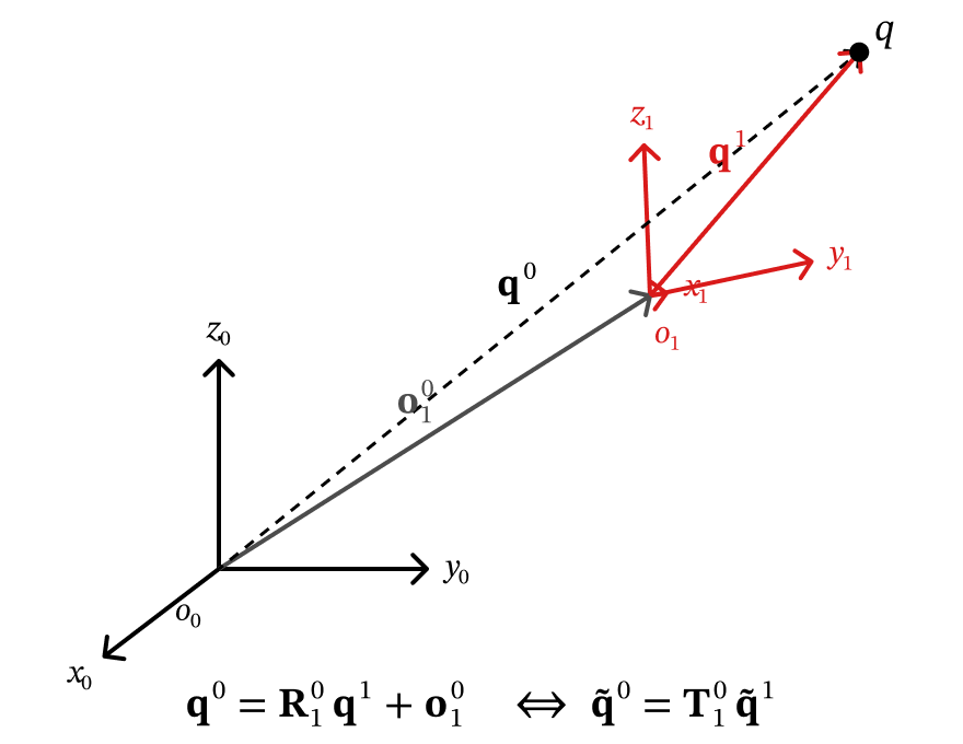
Figure 4.14 — The 3D HTM moves a point from frame {1} coordinates to frame {0} coordinates.
Reading an HTM column by column — you can see the whole frame in it:
| Column | What it is |
|---|---|
| 1 | : where points, in frame |
| 2 | : where points |
| 3 | : where points |
| 4 | : where the origin is |
| bottom row | always |
(Chapter 5 calls these four columns .)
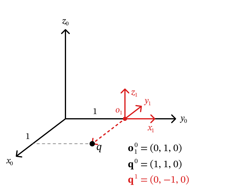
Figure 4.15 — Lecture 7 example: frame {1} at (0, 1, 0), turned 90° about z0.
Worked example (Lecture 7). Frame 's origin is 1 unit along : . Its axes: along , along , along (a turn about ). A point sits at . Its coordinates in frame are (it is 1 unit in the direction from ). Check:
def htm(R, o):
    # 4x4 HTM T_1^0 from the rotation R = R_1^0 and the origin o = o_1^0.
    T = np.eye(4)
    T[:3, :3] = R
    T[:3,  3] = o
    return T


T10 = htm(Rz(np.radians(90)), [0, 1, 0])
q1_tilde = np.array([0, -1, 0, 1])          # [q^1; 1]

print('T_1^0 =\n', T10.round(4))
print('\n[q^0; 1] = T_1^0 [q^1; 1] =', (T10 @ q1_tilde).round(4))
print('\nColumns of T_1^0:  x_1^0 =', T10[:3, 0].round(4), ' y_1^0 =', T10[:3, 1].round(4),
      ' z_1^0 =', T10[:3, 2].round(4), ' o_1^0 =', T10[:3, 3])
T_1^0 =
[[ 0. -1. 0. 0.]
[ 1. 0. 0. 1.]
[ 0. 0. 1. 0.]
[ 0. 0. 0. 1.]]
[q^0; 1] = T_1^0 [q^1; 1] = [1. 1. 0. 1.]
Columns of T_1^0: x_1^0 = [0. 1. 0.] y_1^0 = [-1. 0. 0.] z_1^0 = [0. 0. 1.] o_1^0 = [0. 1. 0.]
4.4.2 Composing HTMs
Chaining frames is matrix multiplication, exactly as in 2D:
is the posture of frame relative to . The inner indices match and “cancel” ( is once a subscript and once a superscript) — a quick way to check that you multiplied in the right order. For a robot arm: .
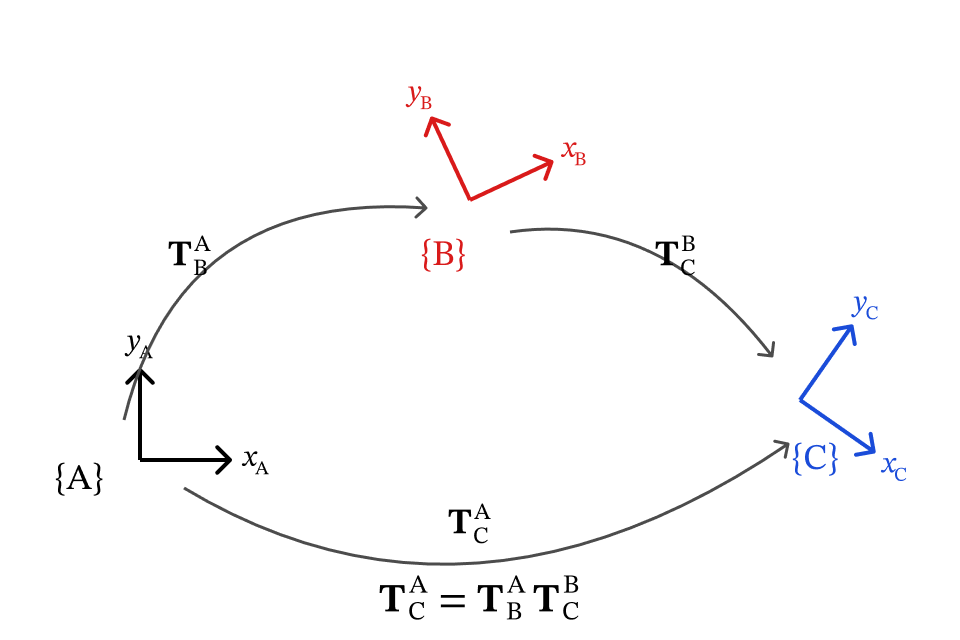
Figure 4.16 — Composing HTMs: the inner indices cancel.
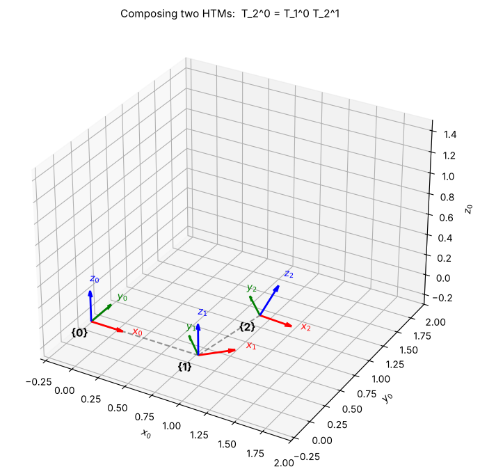
Example: frame is turned about with origin ; frame is turned about with origin in frame .
T10 = htm(Rz(np.radians(45)), [1.0, 0.0, 0.0])     # frame {1} relative to frame {0}
T21 = htm(Ry(np.radians(30)), [0.5, 0.0, 0.3])     # frame {2} relative to frame {1}
T20 = T10 @ T21                                    # frame {2} relative to frame {0}

print('T_1^0 =\n', T10.round(4))
print('\nT_2^1 =\n', T21.round(4))
print('\nT_2^0 = T_1^0 T_2^1 =\n', T20.round(4))

fig = plt.figure(figsize=(8, 7))
ax = fig.add_subplot(111, projection='3d')
for T, name in [(np.eye(4), '0'), (T10, '1'), (T20, '2')]:
    draw_frame_3d(ax, T[:3, :3], T[:3, 3], name=name, scale=0.3)
    ax.text(*(T[:3, 3] - 0.12), '{' + name + '}', fontsize=11, fontweight='bold')
origins = [T[:3, 3] for T in (np.eye(4), T10, T20)]
for a, b in zip(origins[:-1], origins[1:]):
    ax.plot(*zip(a, b), 'k--', alpha=0.4, lw=1.5)
ax.set_xlim(-0.3, 2.0); ax.set_ylim(-0.3, 2.0); ax.set_zlim(-0.3, 1.5)
ax.set_xlabel('$x_0$'); ax.set_ylabel('$y_0$'); ax.set_zlabel('$z_0$')
ax.set_title('Composing two HTMs:  T_2^0 = T_1^0 T_2^1', fontsize=11)
plt.tight_layout(); plt.show()
T_1^0 =
[[ 0.7071 -0.7071 0. 1. ]
[ 0.7071 0.7071 0. 0. ]
[ 0. 0. 1. 0. ]
[ 0. 0. 0. 1. ]]
T_2^1 =
[[ 0.866 0. 0.5 0.5 ]
[ 0. 1. 0. 0. ]
[-0.5 0. 0.866 0.3 ]
[ 0. 0. 0. 1. ]]
T_2^0 = T_1^0 T_2^1 =
[[ 0.6124 -0.7071 0.3536 1.3536]
[ 0.6124 0.7071 0.3536 0.3536]
[-0.5 0. 0.866 0.3 ]
[ 0. 0. 0. 1. ]]
4.4.3 The inverse of an HTM
describes frame seen from frame . You don’t need a general matrix inverse. Start from and solve for : subtract , then multiply by (the inverse of a rotation):
Careful: the top-right block is not just . The offset has to be re-expressed in frame 's directions too.
def htm_inv(T):
    # Inverse of an HTM using R^T (no general matrix inversion).
    R, o = T[:3, :3], T[:3, 3]
    return htm(R.T, -R.T @ o)


T10 = htm(Rz(np.radians(90)), [0, 1, 0])          # the worked example of 4.4.1
T01 = htm_inv(T10)
print('T_0^1 = (T_1^0)^-1 =\n', T01.round(4))
print('\nSame as np.linalg.inv?', np.allclose(T01, np.linalg.inv(T10)))
print('T_1^0 T_0^1 = I ?      ', np.allclose(T10 @ T01, np.eye(4)))
print('\n[q^1; 1] = T_0^1 [q^0; 1] =', T01 @ np.array([1, 1, 0, 1]), '  (expected [0, -1, 0, 1])')
T_0^1 = (T_1^0)^-1 =
[[ 0. 1. 0. -1.]
[-1. 0. 0. -0.]
[ 0. 0. 1. 0.]
[ 0. 0. 0. 1.]]
Same as np.linalg.inv? True
T_1^0 T_0^1 = I ? True
[q^1; 1] = T_0^1 [q^0; 1] = [ 0. -1. 0. 1.] (expected [0, -1, 0, 1])
4.4.4 Explore an HTM
Set the origin and the orientation (as ZYX yaw–pitch–roll) of frame . The black point is fixed in frame at — half a unit along — so it rides along with the frame. Its frame- coordinates are computed with .
def htm_explorer(o_x, o_y, o_z, yaw_deg, pitch_deg, roll_deg):
    o10 = np.array([o_x, o_y, o_z])
    R10 = Rz(np.radians(yaw_deg)) @ Ry(np.radians(pitch_deg)) @ Rx(np.radians(roll_deg))
    T10 = htm(R10, o10)
    q1 = np.array([0.5, 0, 0])
    q0 = (T10 @ np.append(q1, 1))[:3]

    fig = plt.figure(figsize=(9, 7))
    ax = fig.add_subplot(111, projection='3d')
    draw_frame_3d(ax, np.eye(3), name='0', scale=0.6, alpha=0.6)
    draw_frame_3d(ax, R10, o10, name='1', scale=0.6)
    ax.plot(*zip(np.zeros(3), o10), 'k--', alpha=0.35, lw=1.5)
    ax.scatter(*q0, color='black', s=60)
    ax.text(*(q0 + 0.1), 'q', fontsize=12, fontweight='bold')
    setup_3d(ax, 2.0, 'Frame {1} relative to frame {0}')
    plt.tight_layout(); plt.show()
    print('T_1^0 =\n', T10.round(4))
    print('\nq^1 =', q1, '   ->   q^0 =', q0.round(4))


interact(htm_explorer,
         o_x=FloatSlider(value=1.0, min=-1.5, max=1.5, step=0.1, description='o_x'),
         o_y=FloatSlider(value=0.5, min=-1.5, max=1.5, step=0.1, description='o_y'),
         o_z=FloatSlider(value=0.5, min=-1.5, max=1.5, step=0.1, description='o_z'),
         yaw_deg  =FloatSlider(value=30, min=-180, max=180, step=5, description='Yaw ψ (z)'),
         pitch_deg=FloatSlider(value=20, min=-90,  max=90,  step=5, description='Pitch θ (y)'),
roll_deg =FloatSlider(value=10, min=-180, max=180, step=5, description='Roll φ (x)'));Key Takeaways — Section 4.4
(): its columns are .
Transform points with a single multiply: .
Chain frames: (inner indices cancel).
Invert without a general inverse: .
4.5 Chapter Summary and Practice
Cheat sheet
| What | 2D | 3D |
|---|---|---|
| Rotation matrix | , | , |
| Convert a point (same origin) | same | |
| Go back | same | |
| Moved + turned frame | same | |
| HTM | , | same blocks, |
| Transform a point | same | |
| Chain frames | same | |
| Combine rotations | order doesn’t matter | order matters; right = current axes |
Looking ahead. Chapter 5 adds two things: six basic HTMs (, , , , , — the pure translations and the HTM versions of , , ), and a three-step recipe that uses them to write for any robot arm.
Practice problems
Try each one on paper first, then expand the answer or check it with the code cell below.
P1 (2D HTM). Frame has origin and is turned by . A point has . Find .
Answer
\mathbf{R}_1^0 = \begin{bmatrix}0&-1\\1&0\end{bmatrix}, so \mathbf{q}^0 = \mathbf{R}_1^0\mathbf{q}^1 + \mathbf{o}_1^0 = (0, 1) + (2, 0) = (2, 1).
P2 (3D rotation matrix). points along , points along . Where does point? Write and .
Answer
\mathbf{z}_1^0 = \mathbf{x}_1^0\times\mathbf{y}_1^0 = (0,-1,0)\times(1,0,0) = (0,0,1), so z_1 points along z_0. \mathbf{R}_1^0 = \begin{bmatrix}0&1&0\\-1&0&0\\0&0&1\end{bmatrix} = \mathbf{R}_z(-90^\circ), \ \mathbf{R}_0^1 = (\mathbf{R}_1^0)^\top = \begin{bmatrix}0&-1&0\\1&0&0\\0&0&1\end{bmatrix}.
P3 (order of rotations). A frame is first turned about , then about its own new axis. Write the total rotation as a product of basic rotation matrices. Then do the same if the second turn is about the fixed axis.
Answer
Current (own) axis → multiply on the right: \mathbf{R} = \mathbf{R}_z(90^\circ)\,\mathbf{R}_x(90^\circ). Fixed axis → multiply on the left: \mathbf{R} = \mathbf{R}_x(90^\circ)\,\mathbf{R}_z(90^\circ). They are different matrices.
P4 (chaining HTMs). has , . has , . Where is the origin of frame in frame ?
Answer
\mathbf{o}_2^0 = \mathbf{R}_1^0\,\mathbf{o}_2^1 + \mathbf{o}_1^0 = (0, 2, 0) + (1, 0, 0) = (1, 2, 0) — the last column of \mathbf{T}_2^0 = \mathbf{T}_1^0\mathbf{T}_2^1.
# Check your answers to P1-P4
# P1
T10 = htm_2d(np.radians(90), [2, 0])
print('P1: q^0 =', (T10 @ [1, 0, 1])[:2])

# P2
x1, y1 = np.array([0, -1, 0]), np.array([1, 0, 0])
R10 = np.column_stack([x1, y1, np.cross(x1, y1)])
print('\nP2: R_1^0 =\n', R10, '\n    equals R_z(-90°)?', np.allclose(R10, Rz(np.radians(-90))))

# P3
print('\nP3: current axis R_z R_x =\n', (Rz(np.pi/2) @ Rx(np.pi/2)).round(4))
print('    fixed axis   R_x R_z =\n', (Rx(np.pi/2) @ Rz(np.pi/2)).round(4))

# P4
T10 = htm(Rz(np.radians(90)), [1, 0, 0])
T21 = htm(np.eye(3), [2, 0, 0])
print('\nP4: o_2^0 =', (T10 @ T21)[:3, 3].round(4))
P1: q^0 = [2. 1.]
P2: R_1^0 =
[[ 0 1 0]
[-1 0 0]
[ 0 0 1]]
equals R_z(-90°)? True
P3: current axis R_z R_x =
[[ 0. -0. 1.]
[ 1. 0. -0.]
[ 0. 1. 0.]]
fixed axis R_x R_z =
[[ 0. -1. 0.]
[ 0. 0. -1.]
[ 1. 0. 0.]]
P4: o_2^0 = [1. 2. 0.]