In this chapter, we will use the planar 2R robot as a running example to introduce the basic kinematics concepts for robotic systems. The key advantage of working in 2D is that all essential concepts — forward kinematics, inverse kinematics, and velocity kinematics — can be understood using elementary trigonometry before generalizing to 3D in Chapter 4.
The chapter is organized as follows:
Section 3.1 introduces the 2R robot and its parameters.
Section 3.2 solves forward and inverse position kinematics using pure geometry.
Section 3.3 derives velocity kinematics by differentiating the position equations, leading to the Jacobian.
3.1 A 2D Planar Robot
A planar 2R robot has two rigid links connected by two revolute (rotary) joints, with all motion confined to a plane.
Parameters:
| Symbol | Meaning |
|---|---|
| Length of link 1 | |
| Length of link 2 | |
| Angle of joint 1, measured from the positive -axis | |
| Angle of joint 2, measured relative to the direction of link 1 |
Why is relative to link 1, not the global -axis?
Because joint 2 is physically mounted on link 1. When joint 1 rotates, the whole second link rotates with it — so measuring from link 1’s direction captures the actual rotation at that joint. The absolute angle of link 2 in the global frame is .
Key positions:
Base:
Elbow:
End-effector:
In the widget below, the dashed lines show the reference direction each angle is measured from. The arcs show the actual angles.
import numpy as np
import matplotlib.pyplot as plt
import matplotlib.patches as mpatches
%matplotlib inline
def _draw_angle_arc(ax, center, radius, ref_deg, angle_deg, color, label):
"""Draw a labeled arc showing angle_deg measured from the ref_deg direction."""
if abs(angle_deg) < 1.0:
return
a_start = min(ref_deg, ref_deg + angle_deg)
a_end = max(ref_deg, ref_deg + angle_deg)
arc = mpatches.Arc(center, 2*radius, 2*radius,
angle=0, theta1=a_start, theta2=a_end,
color=color, lw=1.8, zorder=4)
ax.add_patch(arc)
mid_rad = np.radians((a_start + a_end) / 2)
ax.text(center[0] + radius * 1.8 * np.cos(mid_rad),
center[1] + radius * 1.8 * np.sin(mid_rad),
label, color=color, fontsize=12, fontweight='bold',
ha='center', va='center')
def draw_2R_robot(theta1_deg, theta2_deg, l1=1.0, l2=0.8, ax=None, show=True):
"""Draw a planar 2R robot given joint angles in degrees."""
theta1 = np.radians(theta1_deg)
theta2 = np.radians(theta2_deg)
p0 = np.array([0.0, 0.0])
p1 = np.array([l1 * np.cos(theta1), l1 * np.sin(theta1)])
p2 = np.array([p1[0] + l2 * np.cos(theta1 + theta2),
p1[1] + l2 * np.sin(theta1 + theta2)])
if ax is None:
fig, ax = plt.subplots(figsize=(6, 6))
# Reference lines (dashed) showing what each angle is measured from
r_ref = 0.42
ax.plot([0, r_ref], [0, 0], color='gray', lw=1, ls='--', zorder=2, alpha=0.8)
ax.plot([p1[0], p1[0] + r_ref * np.cos(theta1)],
[p1[1], p1[1] + r_ref * np.sin(theta1)],
color='gray', lw=1, ls='--', zorder=2, alpha=0.8)
# Angle arcs
_draw_angle_arc(ax, [0.0, 0.0], 0.28, 0, theta1_deg, 'steelblue', 'θ₁')
_draw_angle_arc(ax, [p1[0], p1[1]], 0.20, theta1_deg, theta2_deg, 'tomato', 'θ₂')
# Links
ax.plot([p0[0], p1[0]], [p0[1], p1[1]], color='steelblue', lw=6,
solid_capstyle='round', label=f'Link 1 (l₁ = {l1} m)')
ax.plot([p1[0], p2[0]], [p1[1], p2[1]], color='tomato', lw=6,
solid_capstyle='round', label=f'Link 2 (l₂ = {l2} m)')
# Joints and end-effector
for p in [p0, p1]:
ax.add_patch(plt.Circle(p, 0.05, color='black', zorder=5))
ax.plot(*p2, 'g*', markersize=15, zorder=5, label='End-effector')
ax.annotate('O', p0, xytext=(p0[0] + 0.07, p0[1] - 0.17), fontsize=11)
ax.annotate('p₁', p1, xytext=(p1[0] + 0.07, p1[1] + 0.07), fontsize=11)
ax.set_title(
f'θ₁ = {theta1_deg:.0f}°, θ₂ = {theta2_deg:.0f}° → '
f'EE = ({p2[0]:.3f}, {p2[1]:.3f}) m', fontsize=12)
r = l1 + l2 + 0.3
ax.set_xlim(-r, r); ax.set_ylim(-r, r)
ax.set_aspect('equal'); ax.grid(True, alpha=0.3)
ax.axhline(0, color='gray', lw=0.5); ax.axvline(0, color='gray', lw=0.5)
ax.legend(loc='upper right'); ax.set_xlabel('x (m)'); ax.set_ylabel('y (m)')
if show:
plt.tight_layout(); plt.show()
return p2
# Static snapshot at the default angles (θ₁=45°, θ₂=60°).
# The live notebook version of this cell lets you sweep θ₁/θ₂ with sliders;
# download the notebook and run it locally to explore that interactively.
draw_2R_robot(45, 60);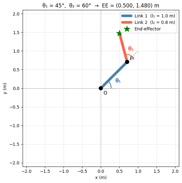
Key Takeaways — Section 3.1
The 2R robot has four parameters: , , , .
is measured relative to link 1, not the global -axis. The absolute angle of link 2 is .
The reachable workspace is an annulus: inner radius , outer radius .
3.2 Position Kinematics
Position kinematics addresses two complementary problems:
Forward kinematics (FK): Given , find the end-effector position .
Inverse kinematics (IK): Given desired , find .
FK is always unique and straightforward. IK is more challenging — for the 2R robot there are generally two solutions for each reachable target, corresponding to the elbow-down and elbow-up configurations.
3.2.1 Forward Kinematics
The end-effector position is found by summing the vector contribution of each link.
Link 1 has length and points at angle from the -axis.
Link 2 has length and points at angle from the -axis (because is measured from link 1, which is already rotated by ).
Sanity check: Set , . Both links point straight up, so we expect , . Plugging in: ✓, ✓.
def forward_kinematics(theta1, theta2, l1=1.0, l2=0.8):
    """
    Forward kinematics for the planar 2R robot.
    theta1, theta2 : joint angles in radians
    Returns (x, y) end-effector position.
    """
    x = l1 * np.cos(theta1) + l2 * np.cos(theta1 + theta2)
    y = l1 * np.sin(theta1) + l2 * np.sin(theta1 + theta2)
    return x, y


# Numerical example
theta1 = np.radians(45)
theta2 = np.radians(60)
x, y = forward_kinematics(theta1, theta2)
print(f'θ₁ = 45°, θ₂ = 60°  →  End-effector: ({x:.4f}, {y:.4f}) m')

# Sanity checks: manually verify a few obvious configurations
print('\nSanity checks:')
sanity = [
    (  0,   0, 'Both links along +x  →  expect (1.8, 0.0)'),
    ( 90,   0, 'Both links straight up  →  expect (0.0, 1.8)'),
    (  0, 180, 'Link 2 folds back  →  expect (0.2, 0.0)  [= l₁−l₂]'),
    ( 90, -90, 'Link 2 points in +x at elbow  →  expect (0.8, 1.0)'),
]
for t1d, t2d, desc in sanity:
    xv, yv = forward_kinematics(np.radians(t1d), np.radians(t2d))
    print(f'  θ₁={t1d:4d}°, θ₂={t2d:4d}°:  ({xv:.4f}, {yv:.4f})   {desc}')
θ₁ = 45°, θ₂ = 60° → End-effector: (0.5001, 1.4798) m
Sanity checks:
θ₁= 0°, θ₂= 0°: (1.8000, 0.0000) Both links along +x → expect (1.8, 0.0)
θ₁= 90°, θ₂= 0°: (0.0000, 1.8000) Both links straight up → expect (0.0, 1.8)
θ₁= 0°, θ₂= 180°: (0.2000, 0.0000) Link 2 folds back → expect (0.2, 0.0) [= l₁−l₂]
θ₁= 90°, θ₂= -90°: (0.8000, 1.0000) Link 2 points in +x at elbow → expect (0.8, 1.0)
Workspace of the Planar 2R Robot
The workspace is the set of all end-effector positions (x,y) the robot can reach as its joints move through their allowed angles.
For the 2R planar robot in this notebook (l_1=1.0), (l_2=0.8):
Maximum reach (arm fully stretched):
Minimum reach (arm folded back):
So the reachable region is an annulus (ring) centered at the base:
In the code below, plot_workspace() samples many (,) pairs, computes FK points (X,Y), and visualizes this ring-shaped reachable set with inner and outer boundary circles.
def plot_workspace(l1=1.0, l2=0.8, n=400):
    """Visualise the reachable workspace of the 2R robot."""
    theta = np.linspace(-np.pi, np.pi, n)
    T1, T2 = np.meshgrid(theta, theta)
    X = l1 * np.cos(T1) + l2 * np.cos(T1 + T2)
    Y = l1 * np.sin(T1) + l2 * np.sin(T1 + T2)

    fig, ax = plt.subplots(figsize=(6, 6))
    ax.scatter(X.ravel(), Y.ravel(), s=0.4, alpha=0.03, color='steelblue')

    phi = np.linspace(0, 2 * np.pi, 300)
    for r, label, ls in [
        (l1 + l2,       f'Outer: r = l₁+l₂ = {l1+l2:.1f} m',       '-'),
        (abs(l1 - l2),  f'Inner: r = |l₁−l₂| = {abs(l1-l2):.1f} m', '--')
    ]:
        ax.plot(r * np.cos(phi), r * np.sin(phi), 'k', ls=ls, lw=1.5, label=label)

    ax.set_aspect('equal');  ax.grid(True, alpha=0.3)
    ax.set_title('Reachable Workspace of the 2R Robot', fontsize=13)
    ax.set_xlabel('x (m)');  ax.set_ylabel('y (m)');  ax.legend()
    plt.tight_layout();  plt.show()


plot_workspace()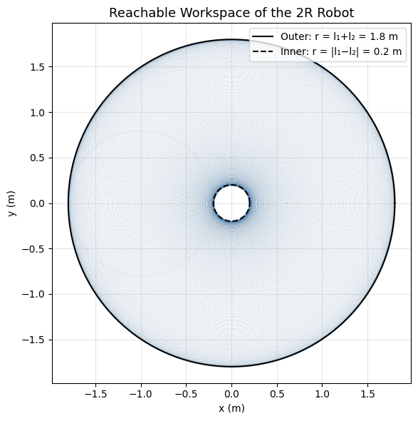
Key Takeaways — Section 3.2.1
FK just sums the two link vectors: , same for .
The absolute angle of link 2 in the global frame is , not .
The workspace is an annulus with inner radius and outer radius .
Math Tool: atan2
The inverse kinematics derivation uses atan2(y, x) rather than the ordinary atan(y/x). Here is why:
atan(y/x)only returns values in and fails when .atan2(y, x)returns the angle of the vector in the full range , correctly handling all four quadrants.
atan2(y, x) | result |
|---|---|
atan2(0, 1) | 0° |
atan2(1, 0) | 90° |
atan2(0, -1) | 180° |
atan2(-1, 0) | -90° |
atan2(1, 1) | 45° |
atan2(1, -1) | 135° |
atan2(-1, 1) | -45° |
# atan2 demonstration
print('atan2(y, x) returns the angle of the vector (x, y) in [-180°, +180°]:\n')
cases = [(0, 1), (1, 0), (0, -1), (-1, 0), (1, 1), (-1, 1), (1, -1)]
for y_val, x_val in cases:
    angle = np.degrees(np.arctan2(y_val, x_val))
    print(f'  atan2({y_val:2d}, {x_val:2d}) = {angle:7.1f}°')

print()
print('Compare with atan(y/x) — wrong quadrant when x < 0:')
for y_val, x_val in [(-1, -1), (1, -1)]:
    atan2_val = np.degrees(np.arctan2(y_val, x_val))
    atan_val  = np.degrees(np.arctan(y_val / x_val))
    print(f'  y={y_val:2d}, x={x_val:2d}:  atan2 = {atan2_val:.1f}°  (correct),  '
          f'atan = {atan_val:.1f}°  (wrong quadrant)')
atan2(y, x) returns the angle of the vector (x, y) in [-180°, +180°]:
atan2( 0, 1) = 0.0°
atan2( 1, 0) = 90.0°
atan2( 0, -1) = 180.0°
atan2(-1, 0) = -90.0°
atan2( 1, 1) = 45.0°
atan2(-1, 1) = -45.0°
atan2( 1, -1) = 135.0°
Compare with atan(y/x) — wrong quadrant when x < 0:
y=-1, x=-1: atan2 = -135.0° (correct), atan = 45.0° (wrong quadrant)
y= 1, x=-1: atan2 = 135.0° (correct), atan = -45.0° (wrong quadrant)
3.2.2 Inverse Kinematics
Physical picture first: Think of the base, elbow, and end-effector as a triangle. The side lengths are , , and (distance from base to target). The angle at the base of this triangle depends on , , — but not on the direction to the target. This means we can find from the distance alone, then find using the direction. There are two triangles for the same side lengths (flip the elbow), giving the two solutions.
Step 1 — Find
Square and add the FK equations:
Expanding (cross terms use the cosine-subtraction identity ):
Solving:
Since , there are two solutions for (positive and negative square root):
Reachability: If the target is outside the workspace — no solution exists.
Step 2 — Find
With known, define:
Then:
The two values of (positive/negative) give two values of , yielding the elbow-down and elbow-up solutions.
def inverse_kinematics(x, y, l1=1.0, l2=0.8):
    """
    Inverse kinematics for the 2R robot.
    Returns list of (theta1, theta2) solutions in radians:
      index 0 = elbow-down (+sin theta2)
      index 1 = elbow-up   (-sin theta2)
    Returns empty list if target is unreachable.
    """
    c2 = (x**2 + y**2 - l1**2 - l2**2) / (2 * l1 * l2)   # cos(theta2)

    if abs(c2) > 1.0:
        print(f'Target ({x:.3f}, {y:.3f}) is outside the workspace.')
        return []

    solutions = []
    for sign in [+1, -1]:                                   # elbow-down, elbow-up
        s2     = sign * np.sqrt(1 - c2**2)                  # sin(theta2)
        theta2 = np.arctan2(s2, c2)                         # theta2 in (-pi, pi]
        alpha  = np.arctan2(y, x)                           # direction to target
        beta   = np.arctan2(l2 * s2, l1 + l2 * c2)         # correction from link 2
        theta1 = alpha - beta
        solutions.append((theta1, theta2))

    return solutions


# Verify: apply FK to each IK solution and check it recovers the target
target = (1.0, 0.8)
sols = inverse_kinematics(*target)

print(f'Target: {target}')
for i, (t1, t2) in enumerate(sols):
    label = 'Elbow-down' if i == 0 else 'Elbow-up  '
    xc, yc = forward_kinematics(t1, t2)
    print(f'  {label}: θ₁={np.degrees(t1):7.2f}°,  θ₂={np.degrees(t2):7.2f}°  '
          f'→  FK check ({xc:.4f}, {yc:.4f})')
Target: (1.0, 0.8)
Elbow-down: θ₁= 0.00°, θ₂= 90.00° → FK check (1.0000, 0.8000)
Elbow-up : θ₁= 77.32°, θ₂= -90.00° → FK check (1.0000, 0.8000)
def ik_interactive(target_x, target_y):
    l1, l2 = 1.0, 0.8
    sols = inverse_kinematics(target_x, target_y, l1, l2)

    fig, axes = plt.subplots(1, 2, figsize=(12, 5))
    config_labels = ['Elbow-down', 'Elbow-up']
    colors = ['steelblue', 'darkorange']

    for ax, label, color in zip(axes, config_labels, colors):
        if not sols:
            ax.text(0.5, 0.5, 'Outside workspace',
                    ha='center', va='center', transform=ax.transAxes, fontsize=13)
        else:
            idx = config_labels.index(label)
            t1, t2 = sols[idx]
            p0 = np.array([0.0, 0.0])
            p1 = np.array([l1*np.cos(t1), l1*np.sin(t1)])
            p2 = np.array([p1[0] + l2*np.cos(t1+t2), p1[1] + l2*np.sin(t1+t2)])

            ax.plot([p0[0], p1[0]], [p0[1], p1[1]], color=color, lw=6, solid_capstyle='round')
            ax.plot([p1[0], p2[0]], [p1[1], p2[1]], color=color, lw=6, solid_capstyle='round', alpha=0.6)
            for p in [p0, p1]:
                ax.add_patch(plt.Circle(p, 0.04, color='black', zorder=5))
            ax.plot(*p2, 'g*', markersize=12, zorder=5, label='EE')
            ax.plot(target_x, target_y, 'rx', ms=14, mew=2.5, label='Target')
            ax.set_title(f'{label}\nθ₁={np.degrees(t1):.1f}°,  θ₂={np.degrees(t2):.1f}°', fontsize=12)
            ax.legend(loc='upper right')

        r = l1 + l2 + 0.2
        ax.set_xlim(-r, r);  ax.set_ylim(-r, r)
        ax.set_aspect('equal');  ax.grid(True, alpha=0.3)
        ax.axhline(0, color='gray', lw=0.5);  ax.axvline(0, color='gray', lw=0.5)

    plt.suptitle(f'IK: Target = ({target_x:.2f}, {target_y:.2f}) m', fontsize=13)
    plt.tight_layout();  plt.show()


# Static snapshot at the default target (x=1.0 m, y=0.8 m).
# The live notebook version of this cell lets you drag the target with sliders;
# download the notebook and run it locally to explore that interactively.
ik_interactive(1.0, 0.8)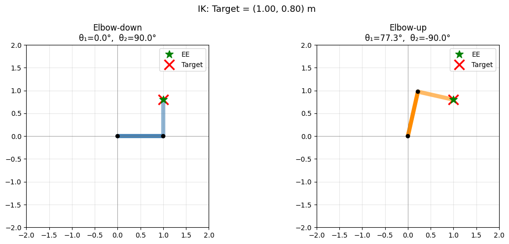
Key Takeaways — Section 3.2.2
Squaring and adding the FK equations eliminates and gives a direct formula for .
Two solutions exist because (elbow-down and elbow-up).
Once is known, where accounts for link 2’s offset.
Use
atan2, notatan, to handle all quadrants correctly.
Practice Problems — Section 3.2
Compute FK for , , , . Verify with the code.
Is the target reachable? Find both IK solutions and confirm with FK.
What happens to the inner workspace radius when ? What does this mean for IK at that boundary?
Try an unreachable target in
ik_interactive. Where exactly is the boundary between reachable and unreachable?
3.3 Velocity Kinematics
The Jacobian relates the joint velocities to the end-effector’s velocity. Specifically, it answers the question “if the joints rotate at certain speeds, how fast does the end-effector move?” It is the matrix that linearly maps joint velocities to end-effector velocity . Like all derivatives, it is only valid instantaneously at the current configuration — the robot’s shape changes the relationship.
Differentiating the FK equations with respect to time (chain rule):
In matrix form:
Column interpretation: Each column of is the end-effector velocity produced when only that joint moves at 1 rad/s:
Column 1 (): both links swing with joint 1, so the EE velocity has contributions from both.
Column 2 (): only link 2 swings, so only link 2 contributes.
Singularities: .
This is zero when (arm fully extended) or (arm fully folded back). At these configurations the two links are collinear and the robot cannot move the end-effector perpendicular to that line — it has temporarily lost one degree of freedom.
def jacobian(theta1, theta2, l1=1.0, l2=0.8):
    """Analytic Jacobian of the 2R robot (2x2 matrix)."""
    s1  = np.sin(theta1)
    c1  = np.cos(theta1)
    s12 = np.sin(theta1 + theta2)
    c12 = np.cos(theta1 + theta2)
    return np.array([
        [-l1*s1 - l2*s12,  -l2*s12],
        [ l1*c1 + l2*c12,   l2*c12]
    ])


theta1, theta2 = np.radians(45), np.radians(60)
J = jacobian(theta1, theta2)

print('Jacobian at θ₁=45°, θ₂=60°:')
print(J.round(4))

# Column interpretation
print('\nColumn interpretation:')
v_col1 = J @ np.array([1.0, 0.0])
v_col2 = J @ np.array([0.0, 1.0])
print(f'  Only θ̇₁=1 rad/s  →  EE velocity = {v_col1.round(4)} m/s  (= col 1 of J)')
print(f'  Only θ̇₂=1 rad/s  →  EE velocity = {v_col2.round(4)} m/s  (= col 2 of J)')

# Full example
dtheta = np.array([0.5, -0.3])
v_ee   = J @ dtheta
print(f'\nWith θ̇₁=0.5, θ̇₂=-0.3 rad/s  →  EE velocity = {v_ee.round(4)} m/s')

print(f'\ndet(J) = {np.linalg.det(J):.4f}')
print(f'l₁ l₂ sin(θ₂) = {1.0 * 0.8 * np.sin(theta2):.4f}  (should match)')

# Physical meaning: write J by its columns, J = [J1  J2]. Then
#   v_ee = J @ dtheta = J1*dtheta1 + J2*dtheta2
# J1 and J2 are FIXED DIRECTIONS (they depend only on the configuration, not on the joint
# speeds); dtheta1 and dtheta2 are the MAGNITUDES that scale those directions (and can flip
# them, if negative). The two scaled vectors add tip-to-tail to give the actual EE velocity.
J1, J2 = J[:, 0], J[:, 1]
contrib1 = J1 * dtheta[0]
contrib2 = J2 * dtheta[1]
print(f'\nPhysical meaning — v_ee = J1·θ̇₁ + J2·θ̇₂:')
print(f"  J1 = {J1.round(4)}  (joint 1's direction, |J1| = {np.linalg.norm(J1):.4f})")
print(f"  J2 = {J2.round(4)}  (joint 2's direction, |J2| = {np.linalg.norm(J2):.4f})")
print(f"  J1 · θ̇₁ = {contrib1.round(4)} m/s   (joint 1's contribution)")
print(f"  J2 · θ̇₂ = {contrib2.round(4)} m/s   (joint 2's contribution)")
print(f'  Sum      = {(contrib1 + contrib2).round(4)} m/s   (matches v_ee above ✓)')
Jacobian at θ₁=45°, θ₂=60°:
[[-1.4798 -0.7727]
[ 0.5001 -0.2071]]
Column interpretation:
Only θ̇₁=1 rad/s → EE velocity = [-1.4798 0.5001] m/s (= col 1 of J)
Only θ̇₂=1 rad/s → EE velocity = [-0.7727 -0.2071] m/s (= col 2 of J)
With θ̇₁=0.5, θ̇₂=-0.3 rad/s → EE velocity = [-0.5081 0.3121] m/s
det(J) = 0.6928
l₁ l₂ sin(θ₂) = 0.6928 (should match)
Physical meaning — v_ee = J1·θ̇₁ + J2·θ̇₂:
J1 = [-1.4798 0.5001] (joint 1's direction, |J1| = 1.5620)
J2 = [-0.7727 -0.2071] (joint 2's direction, |J2| = 0.8000)
J1 · θ̇₁ = [-0.7399 0.25 ] m/s (joint 1's contribution)
J2 · θ̇₂ = [0.2318 0.0621] m/s (joint 2's contribution)
Sum = [-0.5081 0.3121] m/s (matches v_ee above ✓)
Physical Meaning: the Jacobian as a Sum of Joint Contributions
Split into its two columns, . The matrix-vector product then reads as a vector sum:
Each term is one joint’s contribution to the end-effector velocity, and each contribution has a clean direction/magnitude split:
is a direction — the vector the end-effector would move along if joint 1 alone spun at 1 rad/s. It depends only on the current configuration , not on how fast the joints are actually moving.
is the magnitude — it stretches, shrinks, or reverses that fixed direction. A negative just flips to point the other way.
Likewise, is joint 2’s contribution: direction , scaled by .
The true end-effector velocity is what you get by placing these two contributions tip-to-tail and drawing the arrow from the start to the final point — ordinary vector addition.
This is exactly what matrix-vector multiplication is, viewed geometrically: scales each column by its matching component of and adds the results. The plot below draws the two contributions tip-to-tail (in steel blue and tomato, matching the link colors) alongside the resultant (dashed purple) for the same numbers used above.
def plot_jacobian_decomposition(theta1_deg, theta2_deg, dtheta1, dtheta2):
    """Visualise v_ee = J1*dtheta1 + J2*dtheta2 as a tip-to-tail vector sum."""
    l1, l2 = 1.0, 0.8
    t1, t2 = np.radians(theta1_deg), np.radians(theta2_deg)

    p0 = np.array([0.0, 0.0])
    p1 = np.array([l1*np.cos(t1), l1*np.sin(t1)])
    p2 = np.array([p1[0] + l2*np.cos(t1+t2), p1[1] + l2*np.sin(t1+t2)])

    J = jacobian(t1, t2, l1, l2)
    J1, J2 = J[:, 0], J[:, 1]
    contrib1 = J1 * dtheta1        # joint 1's contribution: direction J1, magnitude dtheta1
    contrib2 = J2 * dtheta2        # joint 2's contribution: direction J2, magnitude dtheta2
    v_ee = contrib1 + contrib2     # vector sum = J @ [dtheta1, dtheta2]

    fig, (ax_robot, ax_zoom) = plt.subplots(1, 2, figsize=(13, 6.5))

    # ---- Left panel: robot pose, for context ----
    ax_robot.plot([p0[0], p1[0]], [p0[1], p1[1]], color='steelblue', lw=6, solid_capstyle='round')
    ax_robot.plot([p1[0], p2[0]], [p1[1], p2[1]], color='tomato', lw=6, solid_capstyle='round')
    for p in [p0, p1]:
        ax_robot.add_patch(plt.Circle(p, 0.05, color='black', zorder=5))
    ax_robot.plot(*p2, 'go', ms=10, zorder=5)
    r = l1 + l2 + 0.3
    ax_robot.set_xlim(-r, r);  ax_robot.set_ylim(-r, r)
    ax_robot.set_aspect('equal');  ax_robot.grid(True, alpha=0.3)
    ax_robot.axhline(0, color='gray', lw=0.5);  ax_robot.axvline(0, color='gray', lw=0.5)
    ax_robot.set_xlabel('x (m)');  ax_robot.set_ylabel('y (m)')
    ax_robot.set_title(f'θ₁={theta1_deg}°,  θ₂={theta2_deg}°', fontsize=11)

    # ---- Right panel: zoomed-in vector addition at the end-effector ----
    # Joint 1's contribution: J1*dtheta1, drawn starting at the end-effector
    tip1 = p2 + contrib1
    ax_zoom.annotate('', xy=tip1, xytext=p2,
                      arrowprops=dict(arrowstyle='->', color='steelblue', lw=3))
    ax_zoom.text(*(0.5*(p2+tip1) + np.array([-0.05, 0.06])),
                 r'$\mathbf{J}_1\dot\theta_1$', color='steelblue', fontsize=13, fontweight='bold')

    # Joint 2's contribution: J2*dtheta2, drawn tip-to-tail from the end of contribution 1
    tip2 = tip1 + contrib2
    ax_zoom.annotate('', xy=tip2, xytext=tip1,
                      arrowprops=dict(arrowstyle='->', color='tomato', lw=3))
    ax_zoom.text(*(0.5*(tip1+tip2) + np.array([0.03, 0.03])),
                 r'$\mathbf{J}_2\dot\theta_2$', color='tomato', fontsize=13, fontweight='bold')

    # Resultant v_ee, drawn directly from the end-effector -- its tip should land on tip2
    ax_zoom.annotate('', xy=p2 + v_ee, xytext=p2,
                      arrowprops=dict(arrowstyle='->', color='purple', lw=3, ls='--'))
    ax_zoom.text(*(p2 + v_ee + np.array([0.04, -0.10])),
                 f'$\\dot{{\\mathbf{{p}}}}$ = ({v_ee[0]:.2f}, {v_ee[1]:.2f}) m/s',
                 color='purple', fontsize=11, fontweight='bold')

    ax_zoom.plot(*p2, 'go', ms=10, zorder=5, label='End-effector')
    all_pts = np.array([p2, tip1, tip2, p2 + v_ee])
    pad = 0.25
    ax_zoom.set_xlim(all_pts[:, 0].min() - pad, all_pts[:, 0].max() + pad)
    ax_zoom.set_ylim(all_pts[:, 1].min() - pad, all_pts[:, 1].max() + pad)
    ax_zoom.set_aspect('equal');  ax_zoom.grid(True, alpha=0.3)
    ax_zoom.set_xlabel('x (m)');  ax_zoom.set_ylabel('y (m)')
    ax_zoom.set_title(f'Zoomed view at the end-effector:  θ̇₁={dtheta1}, θ̇₂={dtheta2} rad/s',
                       fontsize=11)

    plt.suptitle(r'$\dot{\mathbf{p}} = \mathbf{J}_1\dot\theta_1 + \mathbf{J}_2\dot\theta_2$'
                 ' -- vector addition of the two joint contributions', fontsize=13)
    plt.tight_layout();  plt.show()


# Same configuration and joint speeds as the numeric example above (θ₁=45°, θ₂=60°,
# θ̇₁=0.5, θ̇₂=-0.3 rad/s) -- the dashed resultant should exactly reach the tip of the
# second (tomato) arrow, confirming J1*θ̇1 + J2*θ̇2 = v_ee.
plot_jacobian_decomposition(45, 60, 0.5, -0.3)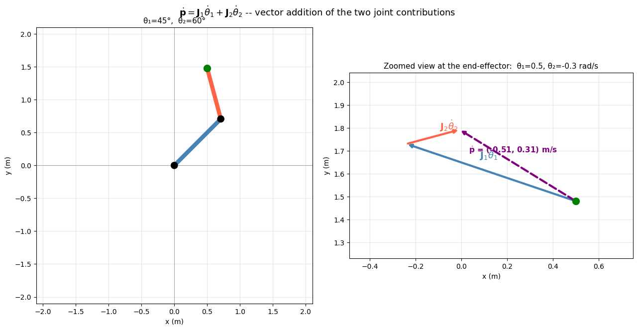
def velocity_interactive(theta1_deg, theta2_deg, dtheta1, dtheta2):
    l1, l2 = 1.0, 0.8
    t1, t2 = np.radians(theta1_deg), np.radians(theta2_deg)

    p0 = np.array([0.0, 0.0])
    p1 = np.array([l1*np.cos(t1), l1*np.sin(t1)])
    p2 = np.array([p1[0]+l2*np.cos(t1+t2), p1[1]+l2*np.sin(t1+t2)])

    J    = jacobian(t1, t2, l1, l2)
    v_ee = J @ np.array([dtheta1, dtheta2])
    detJ = np.linalg.det(J)

    fig, ax = plt.subplots(figsize=(7, 7))
    ax.plot([p0[0],p1[0]], [p0[1],p1[1]], color='steelblue', lw=6, solid_capstyle='round')
    ax.plot([p1[0],p2[0]], [p1[1],p2[1]], color='tomato',    lw=6, solid_capstyle='round')
    for p in [p0, p1]:
        ax.add_patch(plt.Circle(p, 0.05, color='black', zorder=5))
    ax.plot(*p2, 'go', ms=10, zorder=5)

    if np.linalg.norm(v_ee) > 1e-6:
        scale = 0.6
        ax.annotate('', xy=p2+scale*v_ee, xytext=p2,
                    arrowprops=dict(arrowstyle='->', color='purple', lw=2.5))
        ax.text(p2[0]+scale*v_ee[0]+0.05, p2[1]+scale*v_ee[1]+0.05,
                f'v = ({v_ee[0]:.2f}, {v_ee[1]:.2f}) m/s', color='purple', fontsize=10)

    warn = '  ⚠ Near singularity! (θ₂ ≈ 0° or ±180°)' if abs(detJ) < 0.15 else ''
    ax.set_title(f'θ₁={theta1_deg}°,  θ₂={theta2_deg}°  |  det(J)={detJ:.3f}{warn}', fontsize=11)
    r = l1+l2+0.3
    ax.set_xlim(-r,r);  ax.set_ylim(-r,r)
    ax.set_aspect('equal');  ax.grid(True, alpha=0.3)
    ax.axhline(0, color='gray', lw=0.5);  ax.axvline(0, color='gray', lw=0.5)
    ax.set_xlabel('x (m)');  ax.set_ylabel('y (m)')
    plt.tight_layout();  plt.show()


# Static snapshot at the default configuration/velocities.
# The live notebook version of this cell lets you sweep angles and joint velocities with sliders;
# download the notebook and run it locally to explore that interactively.
velocity_interactive(45, 60, 0.5, -0.3)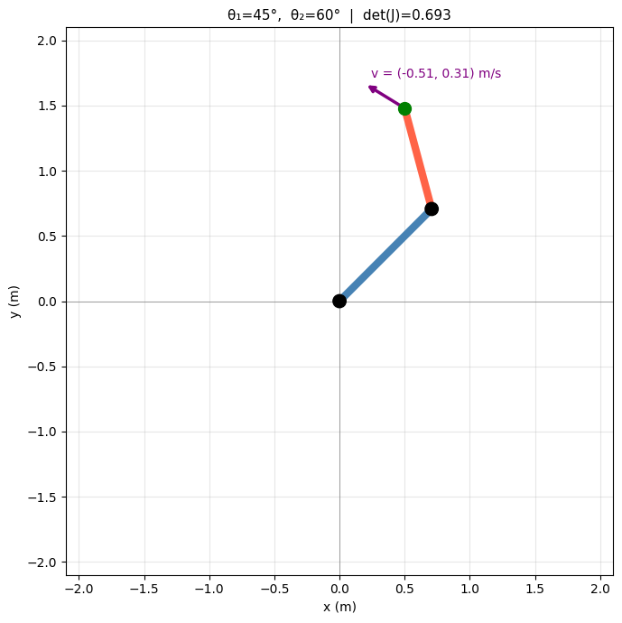
Key Takeaways — Section 3.3
The Jacobian linearly maps joint velocities to end-effector velocity: .
Column of is the EE velocity when only joint rotates at 1 rad/s.
: zero when the arm is fully extended or fully folded.
At a singularity the robot cannot move in one Cartesian direction, no matter what the joints do.
Practice Problems — Section 3.3
At , , compute by hand and verify with the code.
Slide slowly toward in
velocity_interactive. What happens to the velocity arrow and why?Find a configuration where joint 1 rotation produces no -velocity at the end-effector. What does the robot look like?
If the desired EE velocity is , what joint velocities are required at , ? (Hint: compute at that configuration.)
3.4 Simulating the 2R Robot using MuJoCo
MuJoCo is a physics engine widely used for robotics simulation and control. It provides efficient computation of kinematics, dynamics, and collisions. In this section, we use MuJoCo as a kinematics engine — without advancing time, so the physics only computes geometry — to validate the forward kinematics formulas we derived in Sections 3.2 and 3.3. You can find an introductory tutorial here: MuJoCo Tutorial.
We build the same 2R arm ( m, m) defined in MJCF (MuJoCo XML Format). In practice, robot models come from CAD software (SolidWorks, Fusion 360) → STL mesh export → URDF description → MJCF conversion. Here we write the XML by hand so every element is explicit and readable.
Three objects appear throughout every MuJoCo program:
| Object | What it represents |
|---|---|
MjModel | Static robot structure — bodies, joints, geometries, sensors. Loaded once from XML; never changes during a run. |
MjData | Time-varying state — joint angles (qpos), velocities (qvel), body poses (xpos, xmat), forces. |
mj_forward(model, data) | Given angles in data.qpos, propagates the kinematic chain and writes every body’s world-frame position into data.xpos. |
3.4.1 Defining the Robot in MJCF
An MJCF file is a plain-text XML file that describes the robot completely. The elements we need for a 2R arm:
| Element | Role |
|---|---|
<body> | A rigid link. Nest bodies inside each other to form a kinematic chain. |
<joint> | Adds one degree of freedom: how this body moves relative to its parent. For a revolute joint use type="hinge". |
<geom> | A geometric shape (capsule, sphere, box, …) used for rendering and collision. |
<camera> | A virtual viewpoint. We add a top-down camera to view the planar robot from above. |
Kinematic tree — XML nesting mirrors the physical chain:
worldbody
└── link1  ← joint1: hinge around z, relative to world
    └── link2  ← joint2: hinge around z, relative to link1
        └── end_effector  ← rigidly fixed to link2 (no joint)
Key rule: the pos="…" attribute of a <body> sets its origin in its parent’s local frame.
Writing pos="1.0 0 0" for link2 means “my origin is 1 m along link1’s local x-axis” — exactly the elbow.
The code cell below writes out the full MJCF, loads it into MuJoCo, and prints the resulting model structure.
# Install MuJoCo if not already available:
# !pip install mujoco

import mujoco

# MJCF: complete description of the 2R planar robot.
# l1 = 1.0 m,  l2 = 0.8 m  (same as Sections 3.2-3.6)
# The robot moves in the x-y plane; joints rotate about the z-axis.
XML_2R = """
<mujoco model="2R_planar_robot">

  <!-- No gravity: kinematics only -->
  <option gravity="0 0 0"/>

  <!-- ====================================================================
       SCENE APPEARANCE
       visual : global rendering settings (lighting, haze)
       asset  : textures and materials — referenced by geoms via material=""
  ==================================================================== -->
  <visual>
    <!-- headlight = flashlight attached to the camera.
         ambient prevents fully-shadowed areas from being pitch black. -->
    <headlight diffuse="0.5 0.5 0.5" ambient="0.3 0.3 0.3" specular="0.0 0.0 0.0"/>
    <!-- haze blends the far background with this blue-grey colour -->
    <rgba haze="0.15 0.25 0.35 1"/>
  </visual>

  <asset>
    <!-- Two-tone blue checkerboard floor texture.
         builtin="checker" generates the pattern entirely inside MuJoCo —
         no external image file needed.
         rgb1 / rgb2 = the two alternating tile colours. -->
    <texture name="floor_tex" type="2d" builtin="checker"
             rgb1="0.15 0.25 0.38" rgb2="0.22 0.38 0.55"
             width="512" height="512"/>
    <!-- Material wraps the texture and adds surface properties.
         texrepeat="6 6" tiles the checker 6 times per unit length.
         reflectance adds a subtle mirror-like sheen. -->
    <material name="floor_mat" texture="floor_tex" texrepeat="6 6"
              reflectance="0.2" shininess="0.1"/>

    <!-- Gradient skybox: blue at the horizon, dark at the top.
         type="skybox" tells MuJoCo to use this as the scene background. -->
    <texture name="skybox" type="skybox" builtin="gradient"
             rgb1="0.3 0.5 0.7" rgb2="0.05 0.05 0.15"
             width="512" height="512"/>
  </asset>

  <worldbody>

    <!-- Overhead directional light.
         dir points slightly off-axis for a natural look.
         castshadow="true" lets the links cast shadows on the floor. -->
    <light name="sun" pos="1 1 5" dir="-0.2 -0.2 -1"
           diffuse="0.8 0.8 0.8" specular="0.2 0.2 0.2" castshadow="true"/>

    <!-- Infinite ground plane with checker material.
         size="10 10 0.1" sets the half-extents of the rendered area.
         pos z=-0.02 places the floor just below the robot (which lives at z=0). -->
    <geom name="floor" type="plane" size="10 10 0.1" pos="0 0 -0.1"
          material="floor_mat"/>

    <!-- Top-down camera looking straight down the z-axis.
         pos    = (0, 0, 5) -- 5 m above the origin
         xyaxes = camera x-axis then y-axis in world frame;
                  "1 0 0  0 1 0" makes the camera look along -z (downward) -->
    <camera name="top" pos="0 0 5" xyaxes="1 0 0 0 1 0"/>

    <!-- Small cylinder marks the base (joint 1 location) -->
    <geom name="base_marker" type="cylinder" pos="0 0 0"
          size="0.07 0.07" rgba="0.15 0.15 0.15 1"/>

    <!-- =====================================================================
         LINK 1
         pos="0 0 0"  : link1 origin at the world origin
         joint1       : hinge (revolute) around the z-axis
    ===================================================================== -->
    <body name="link1" pos="0 0 0">
      <joint name="joint1" type="hinge" axis="0 0 1" pos="0 0 0"/>

      <!-- Capsule for link 1 (inset slightly so joint markers stay visible) -->
      <geom name="geom_link1" type="capsule"
            fromto="0.06 0 0   0.94 0 0"
            size="0.04" rgba="0.25 0.47 0.80 1"/>

      <!-- Elbow marker at the tip of link 1 -->
      <geom name="elbow_marker" type="cylinder" pos="1.0 0 0"
            size="0.07 0.07" rgba="0.15 0.15 0.15 1"/>

      <!-- ===================================================================
           LINK 2
           pos="1.0 0 0"  : link2 origin at the elbow
           joint2          : hinge around z, relative to link1
      =================================================================== -->
      <body name="link2" pos="1.0 0 0">
        <joint name="joint2" type="hinge" axis="0 0 1" pos="0 0 0"/>

        <!-- Capsule for link 2 (length 0.8 m) -->
        <geom name="geom_link2" type="capsule"
              fromto="0.06 0 0   0.74 0 0"
              size="0.04" rgba="0.80 0.25 0.25 1"/>

        <!-- =================================================================
             END-EFFECTOR
             pos="0.8 0 0"  : tip of link 2, rigidly attached (no joint)
        ================================================================= -->
        <body name="end_effector" pos="0.8 0 0">
          <geom name="ee_marker" type="sphere" size="0.08" rgba="0.0 0.75 0.0 1"/>
        </body>

      </body>   <!-- end link2 -->
    </body>     <!-- end link1 -->

  </worldbody>
</mujoco>
"""

# Load the XML into MuJoCo
model = mujoco.MjModel.from_xml_string(XML_2R)
data  = mujoco.MjData(model)

print("=== Model summary ===")
print(f"  Bodies (including world):  {model.nbody}")
print(f"  Joints:                    {model.njnt}")
print(f"  qpos size:                 {model.nq}")
print()
print("=== Body index — data.xpos[id] gives world-frame (x, y, z) ===")
for i in range(model.nbody):
    name = mujoco.mj_id2name(model, mujoco.mjtObj.mjOBJ_BODY, i)
    print(f"  body[{i}]  '{name}'")
print()

# Look up body IDs by name (safer than hard-coding integers)
ee_id = mujoco.mj_name2id(model, mujoco.mjtObj.mjOBJ_BODY, "end_effector")
l2_id = mujoco.mj_name2id(model, mujoco.mjtObj.mjOBJ_BODY, "link2")
print(f"'end_effector' id = {ee_id}  ->  data.xpos[{ee_id}] = EE world position")
print(f"'link2'        id = {l2_id}  ->  data.xpos[{l2_id}] = elbow world position")
=== Model summary ===
  Bodies (including world):  4
  Joints:                    2
  qpos size:                 2

=== Body index — data.xpos[id] gives world-frame (x, y, z) ===
  body[0]  'world'
  body[1]  'link1'
  body[2]  'link2'
  body[3]  'end_effector'

'end_effector' id = 3  ->  data.xpos[3] = EE world position
'link2'        id = 2  ->  data.xpos[2] = elbow world position
3.4.2 Forward Kinematics with MuJoCo
The MuJoCo FK workflow is always the same three lines — and will look identical whether the robot has 2 joints or 20:
data.qpos[0] = theta1           # 1. write joint angles in radians
data.qpos[1] = theta2
mujoco.mj_forward(model, data)  # 2. propagate the kinematic chain
ee_pos = data.xpos[ee_id]       # 3. read any body's world-frame position
data.xpos is a NumPy array with shape (nbody, 3). After mj_forward, row i holds the (x, y, z) world-frame position of body i’s origin.
The cell below computes the end-effector position for several configurations and compares all three FK methods side by side.
# ── Compare geometric FK solution with MuJoco solution at several joint configurations ──────────────
#
# For each (θ₁, θ₂):
#   • Geometric FK  — trigonometric formulas   (Section 3.2.1)
#   • MuJoCo FK     — set qpos → mj_forward → read xpos

print("End-effector (x, y) in metres — three methods compared:")
print(f"  {'Config':22}  {'Geometric':>16}  {'MuJoCo':>16}  {'Match':>5}")
print("─" * 84)

configs = [(45, 60), (0, 0), (90, 0), (0, 180), (30, -60), (90, -90)]

for t1d, t2d in configs:
    t1 = np.radians(t1d)
    t2 = np.radians(t2d)

    # ── Method 1: Geometric ──────────────────────────────────────────────────
    x_geo, y_geo = forward_kinematics(t1, t2)

    # ── Method 2: MuJoCo ─────────────────────────────────────────────────────
    data.qpos[0] = t1                    # joint 1 angle (radians)
    data.qpos[1] = t2                    # joint 2 angle (radians)
    mujoco.mj_forward(model, data)       # propagate kinematic chain
    ee = data.xpos[ee_id]                # end-effector (x, y, z) in world frame
    # For our planar robot ee[2] ≈ 0 (no z motion); we use only ee[:2]

    # ── Check they all agree to 4 decimal places ─────────────────────────────
    match = (np.allclose([x_geo, y_geo], ee[:2],   atol=1e-4))

    print(f"  θ₁={t1d:4d}°, θ₂={t2d:4d}°"
          f"   ({x_geo:6.3f},{y_geo:6.3f})"
          f"   ({ee[0]:6.3f},{ee[1]:6.3f})"
          f"   {'✓' if match else '✗':>5}")

print()
print("Both methods return the same end-effector position ✓")
print()
print("The advantage of MuJoCo: no re-derivation needed for any new robot —")
print("define the MJCF, load it, and call mj_forward().")
print()
# Bonus: MuJoCo gives us ALL body positions, not just the end-effector.
# For example, here is the elbow position for the first configuration:
data.qpos[0] = np.radians(45)
data.qpos[1] = np.radians(60)
mujoco.mj_forward(model, data)
elbow = data.xpos[l2_id]   # link2's origin = elbow location
print(f"Bonus — elbow (link2 origin) at θ₁=45°, θ₂=60°: "
      f"({elbow[0]:.4f}, {elbow[1]:.4f})  m")
print(f"  Compare with geometric:  l₁·cos(θ₁) = {np.cos(np.radians(45)):.4f},  "
      f"l₁·sin(θ₁) = {np.sin(np.radians(45)):.4f}  ✓")
End-effector (x, y) in metres — three methods compared:
Config Geometric MuJoCo Match
────────────────────────────────────────────────────────────────────────────────────
θ₁= 45°, θ₂= 60° ( 0.500, 1.480) ( 0.500, 1.480) ✓
θ₁= 0°, θ₂= 0° ( 1.800, 0.000) ( 1.800, 0.000) ✓
θ₁= 90°, θ₂= 0° ( 0.000, 1.800) ( 0.000, 1.800) ✓
θ₁= 0°, θ₂= 180° ( 0.200, 0.000) ( 0.200, 0.000) ✓
θ₁= 30°, θ₂= -60° ( 1.559, 0.100) ( 1.559, 0.100) ✓
θ₁= 90°, θ₂= -90° ( 0.800, 1.000) ( 0.800, 1.000) ✓
Both methods return the same end-effector position ✓
The advantage of MuJoCo: no re-derivation needed for any new robot —
define the MJCF, load it, and call mj_forward().
Bonus — elbow (link2 origin) at θ₁=45°, θ₂=60°: (0.7071, 0.7071) m
Compare with geometric: l₁·cos(θ₁) = 0.7071, l₁·sin(θ₁) = 0.7071 ✓
Bonus: A Live 3D Viewer (local only)
mujoco.viewer.launch_passive() opens an actual desktop window that a slider can drive in real time — genuinely interactive, but it needs a local display and a running Python kernel, so it can’t be reproduced on this static page. Download the notebook and run the cell below yourself to try it:
import mujoco.viewer          # requires mujoco >= 2.2.0
from ipywidgets import interact, FloatSlider

# mujoco.viewer.launch_passive() opens a 3D viewer window WITHOUT blocking
# the notebook -- you can keep running cells while the window is open.
#
# Inside the viewer window you can:
#   Left-click + drag    -- rotate the scene
#   Right-click + drag   -- pan
#   Scroll wheel         -- zoom in / out
#   F1                   -- show all keyboard shortcuts
#   Ctrl+M                -- toggle the "Control" panel (built-in joint sliders)
#
# The notebook sliders below also control the joints in real time.
# Each time a slider moves, update_robot() writes the new angles to data.qpos,
# runs mj_forward(), then calls viewer.sync() to redraw the window.

viewer = mujoco.viewer.launch_passive(model, data)
print("MuJoCo viewer opened -- look for a new window on your desktop.")
print("Use the sliders below, or press Ctrl+M in the viewer for its own controls.")


def update_robot(theta1_deg, theta2_deg):
    """Set joint angles, run FK, and push the updated pose to the viewer."""

    # 1. Write joint angles in radians (MuJoCo always uses radians internally)
    data.qpos[0] = np.radians(theta1_deg)   # joint 1
    data.qpos[1] = np.radians(theta2_deg)   # joint 2

    # 2. Propagate the kinematic chain (fills data.xpos with body positions)
    mujoco.mj_forward(model, data)

    # 3. Push the updated state to the viewer so it redraws the window.
    #    viewer.is_running() returns False if the user has closed the window.
    if viewer.is_running():
        viewer.sync()

    # 4. Print the computed end-effector position below the sliders
    ee_pos = data.xpos[ee_id]   # shape (3,) -- (x, y, z) in world frame
    print(f"theta1={theta1_deg:+6.1f} deg  theta2={theta2_deg:+6.1f} deg"
          f"   ->   EE = ({ee_pos[0]:.4f}, {ee_pos[1]:.4f}) m")


interact(update_robot,
         theta1_deg=FloatSlider(value=45, min=-180, max=180, step=1, description='theta1 (deg)'),
         theta2_deg=FloatSlider(value=60, min=-180, max=180, step=1, description='theta2 (deg)'));
Key Takeaways — Section 3.4
An MJCF file describes the robot as a tree of nested
<body>elements. Each<joint>inside a body adds one degree of freedom relative to its parent.
MjModelholds the static robot structure (loaded once).MjDataholds the current state — joint angles inqpos, body positions inxpos, etc.Three-line FK recipe: write angles into
data.qpos→ callmj_forward(model, data)→ readdata.xpos[body_id].MuJoCo’s FK gives the same end-effector positions as our geometric and HTM formulas — it is a more general engine that handles any kinematic tree in 2D or 3D without re-deriving formulas.
In later chapters we will use this same workflow to simulate the SO-ARM 101 (a real 6-joint robot), loading a CAD-derived MJCF file and calling
mj_forwardjust as we do here.